Survival Analysis Case Report - Telecom Customer Churn Prediction

Author: Chen Sijia

Dataset: IBM Telco Customer Churn

Tutorial Link: https://github.com/databricks-industry-solutions/survival-analysis

Environment: PySpark Environment

---

Table of Contents

1. Introduction
2. Data Overview
3. Survival Analysis Methods
4. Kaplan-Meier Survival Analysis
5. Cox Proportional Hazards Model
6. Accelerated Failure Time Model (AFT)
7. Customer Lifetime Value (CLV)
8. Conclusion
9. Business Recommendations
10. Model Limitations
11. Appendix

---

1. Introduction

1.1 What is Survival Analysis?

Survival Analysis is a collection of statistical methods for studying “time-to-event” data. Although originally applied in medicine (studying patient survival time), it is now widely used in:

• Telecommunications: Customer churn prediction
• Manufacturing: Equipment failure prediction
• Finance: Loan default time prediction
• E-commerce: User activation time prediction

1.2 Project Overview

This case uses survival analysis to predict churn time for telecom customers, helping enterprises:

• Identify customers with high churn risk
• Take retention actions at critical time points
• Optimize customer retention strategies

---

2. Data Overview

2.1 Data Source

• Dataset: IBM Telco Customer Churn Dataset
• Original records: 7,043
• Analysis sample size: 3,351 (month-to-month contract + internet service customers)

2.2 Sample Characteristics

Metric	Value
Number of churned customers	1,556
Churn rate	46.4%
Observation time range	0-72 months

---

3. Survival Analysis Methods

3.1 Kaplan-Meier Estimator

Basic Principle:
Non-parametric method to estimate the survival function S(t) = P(T > t)

Formula:
S(t) = ∏(1 - d_j / n_j)

Where:

• d_j: number of events (churns) at time point j
• n_j: number at risk just before time point j

Advantages:

• No distributional assumptions
• Handles censored data
• Intuitive and easy to interpret

Application: Visualize survival curves for different groups, compare differences between groups

3.2 Cox Proportional Hazards Model

Basic Principle:
Semi-parametric model to analyze the effect of multiple covariates on survival time

Model Form:
h(t|X) = h₀(t) × exp(β₁X₁ + … + βₚXₚ)

Where:

• h(t	X): hazard function

• h₀(t): baseline hazard
• β: covariate coefficients
• exp(β): hazard ratio (HR)

Advantages:

• Analyzes multiple factors simultaneously
• No need to specify baseline hazard
• HR < 1 indicates protective factor, HR > 1 indicates risk factor

Application: Identify key factors influencing customer churn

3.3 Accelerated Failure Time (AFT) Model

Basic Principle:
Parametric model assuming covariates accelerate or decelerate survival time

Model Form:
T = exp(β₁X₁ + … + βₚXₚ + σ·ε)

Where:

• T: survival time
• exp(β): time acceleration factor (>1 extends, <1 shortens)
• ε: error term

Advantages:

• Directly predicts survival time
• Handles multiple distributions (Weibull, LogNormal, LogLogistic)

Application: Predict customer churn probability at specific time points

3.4 Log-Rank Test

Basic Principle:
Chi-square test to test whether multiple survival curves are statistically equivalent

Null Hypothesis: No significant difference among survival curves of groups

Application: Verify whether survival curves differ significantly across groups

3.5 Method Comparison

Method	Type	Purpose	Output
KM	Non-parametric	Estimate survival function	Survival probability
Cox	Semi-parametric	Analyze influencing factors	Hazard ratio (HR)
AFT	Parametric	Predict survival time	Time acceleration factor
Log-rank	Non-parametric test	Compare differences between groups	test_statistic, p, -log2(p)

---

4. Kaplan-Meier Survival Analysis

4.1 Analysis Workflow

from lifelines import KaplanMeierFitter
from lifelines.statistics import pairwise_logrank_test

# Overall KM fit
kmf = KaplanMeierFitter()
kmf.fit(telco_pd['tenure'], telco_pd['churn'].astype(float))

# Group KM and log-rank test
def plot_km(col):
    for r in telco_pd[col].unique():
        ix = telco_pd[col] == r
        kmf.fit(telco_pd.loc[ix, 'tenure'], telco_pd.loc[ix, 'churn'], label=r)
        kmf.plot()

def print_logrank(col):
    log_rank = pairwise_logrank_test(telco_pd['tenure'], telco_pd[col], telco_pd['churn'])
    print(log_rank.summary)

# Perform group analysis
for col in categorical_cols:
    plot_km(col)
    print_logrank(col)

4.2 Analysis Results

4.2.1 Overall Survival Curve

• Median survival time: 34 months
• Interpretation: 50% of customers churn within 34 months

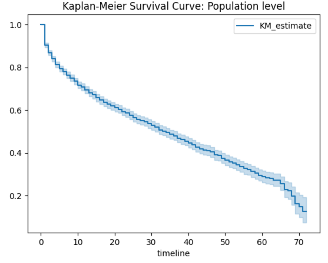Figure 1: Overall Kaplan-Meier survival curve

4.2.2 DSL Internet Service Survival Probability (first 10 months)

Month	DSL Survival Probability
0	1.000000
1	0.902698
2	0.864380
3	0.834702
4	0.810522
5	0.794352
6	0.783900
7	0.776362
8	0.768486
9	0.750833

4.2.3 Group Survival Analysis Results

1. Gender

Metric	Value
test_statistic	2.038938
p-value	0.153317
-log2(p)	2.705414

• Conclusion: p > 0.05, survival curves for different genders are not significantly different

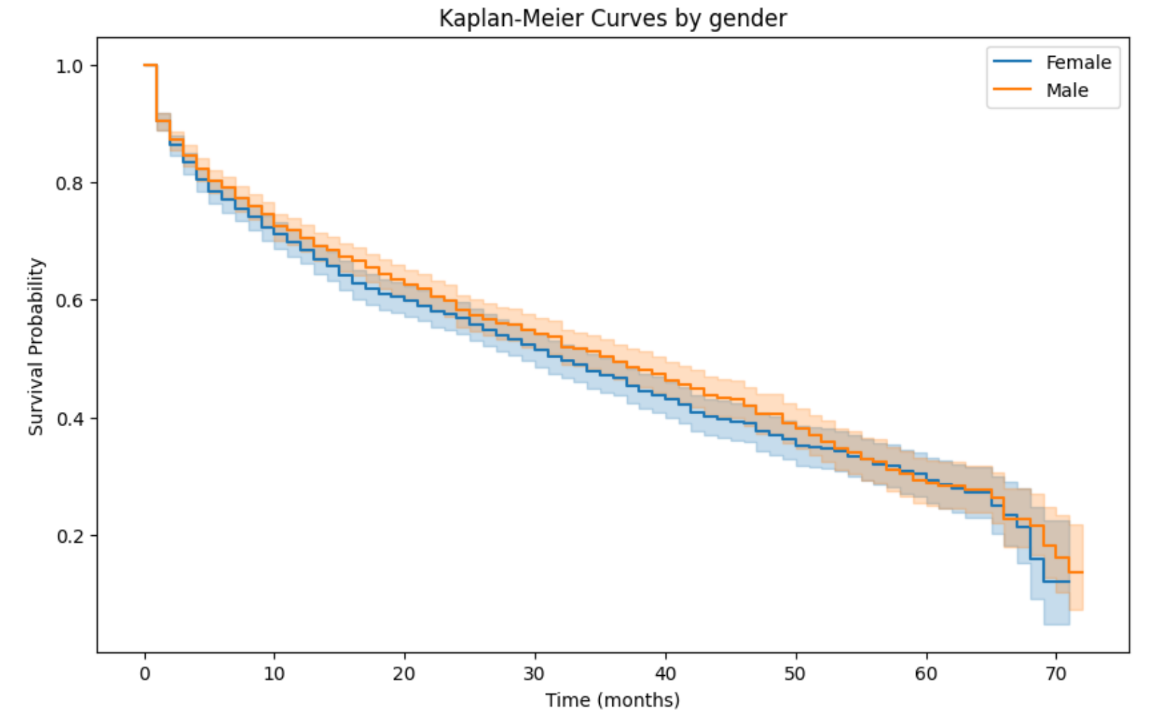Figure 2: Survival curve by gender

---

1. Senior Citizen Status (seniorCitizen)

Metric	Value
test_statistic	0.125471
p-value	0.723174
-log2(p)	0.467584

• Conclusion: p > 0.05, senior citizen status has no significant impact on customer retention

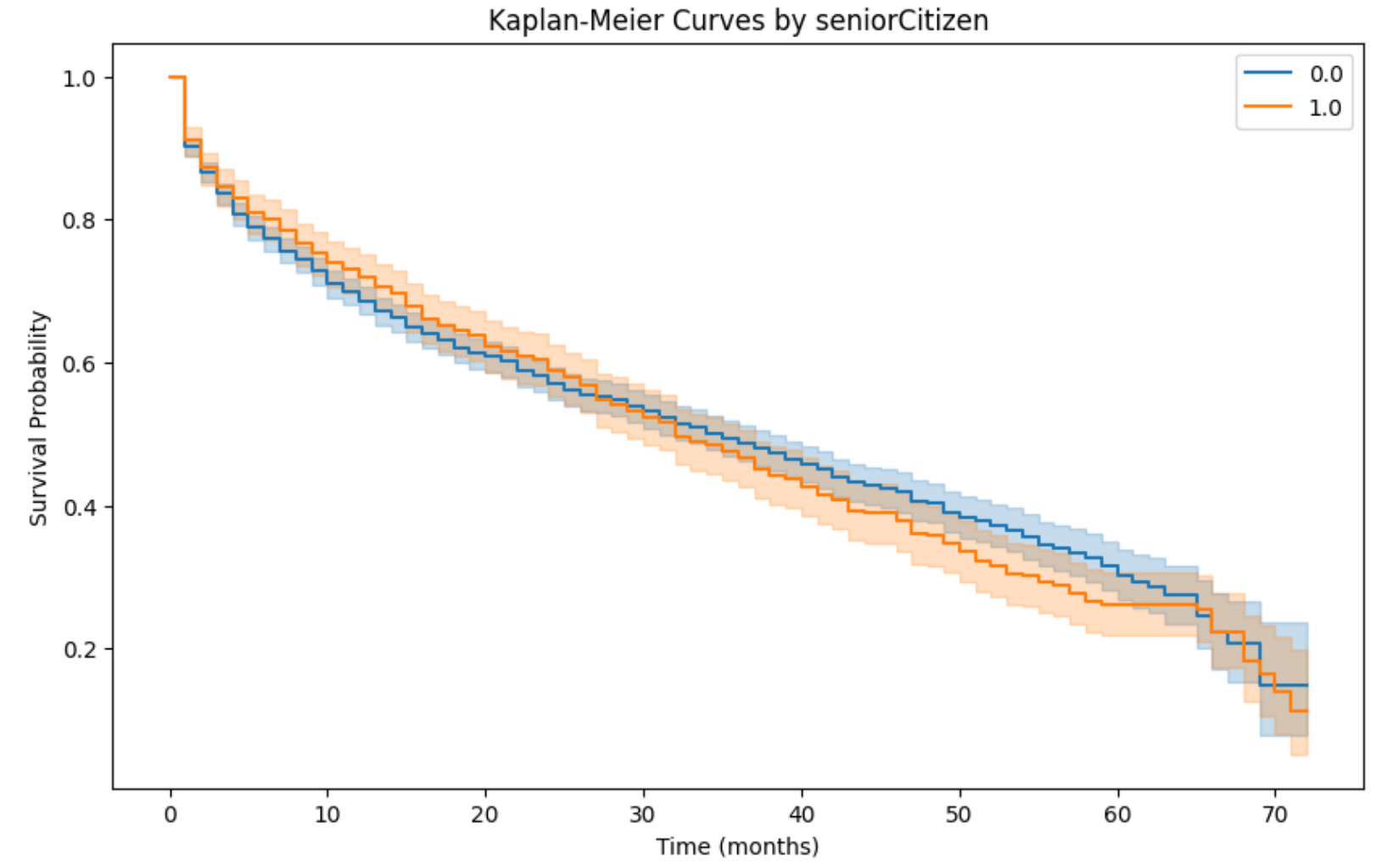Figure 3: Survival curve by senior citizen status

---

1. Partner Status (partner)

Metric	Value
test_statistic	135.758896
p-value	2.252911e-31
-log2(p)	101.807981

• Conclusion: Customers with partners have significantly longer retention time

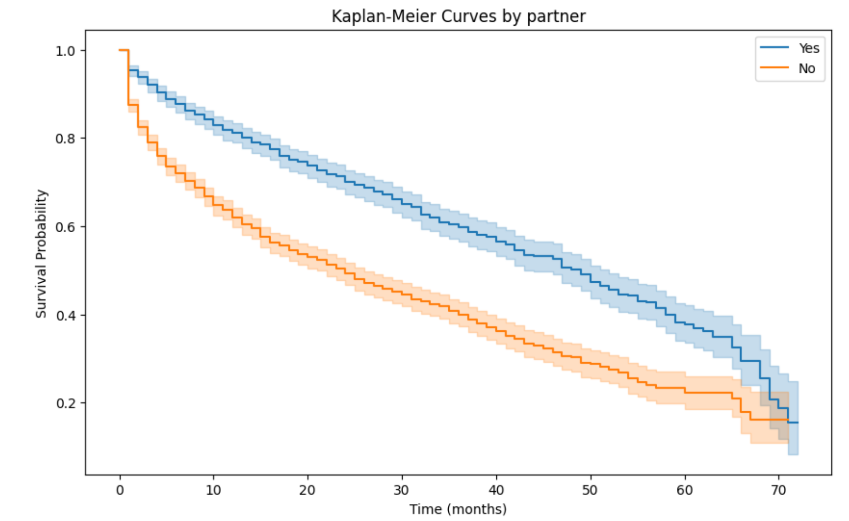Figure 4: Survival curve by partner status

---

1. Dependents Status (dependents)

Metric	Value
test_statistic	35.031241
p-value	3.244576e-09
-log2(p)	28.199323

• Conclusion: Customers with dependents have significantly longer retention time

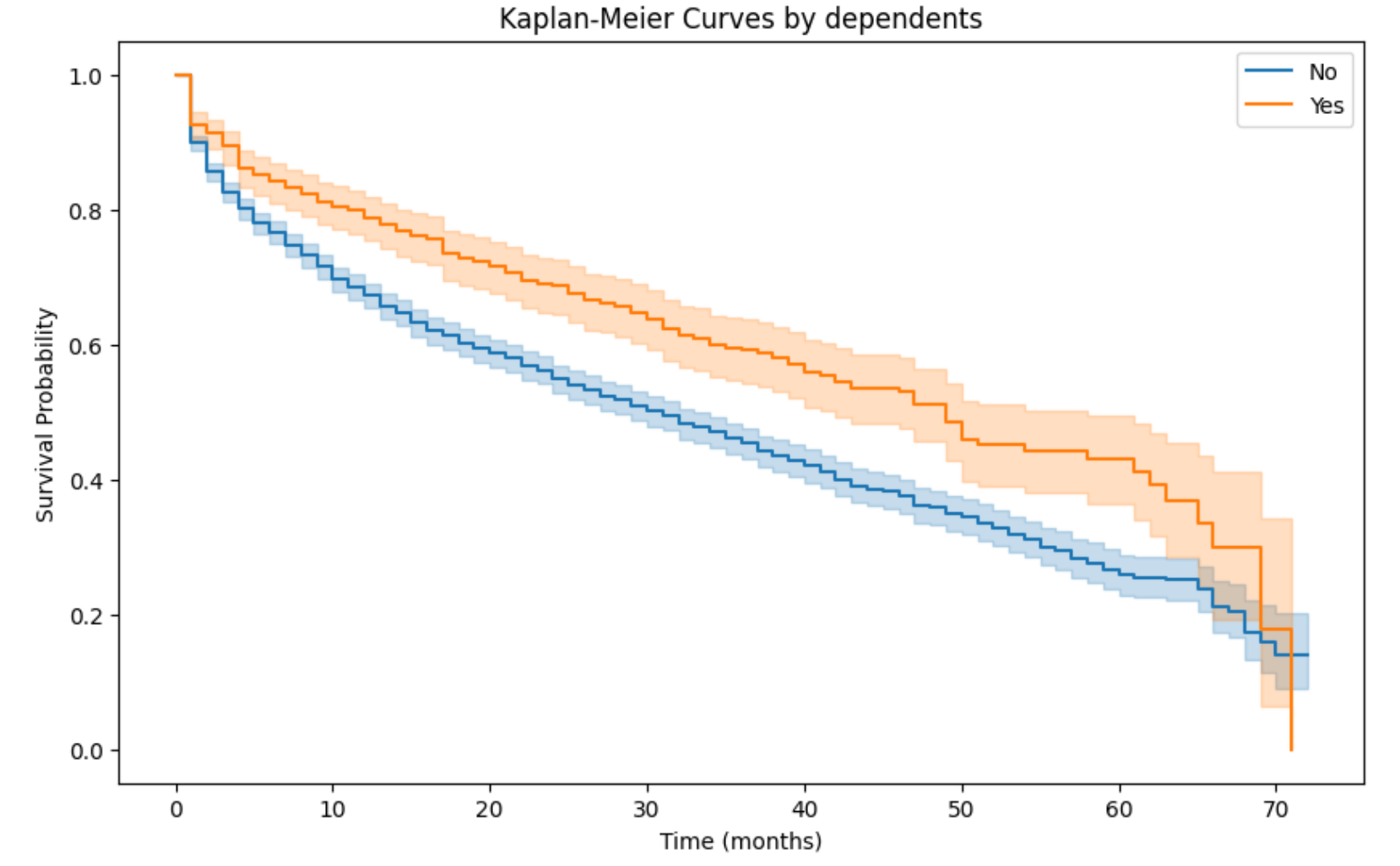Figure 5: Survival curve by dependents status

---

1. Phone Service (phoneService)

Metric	Value
test_statistic	1.683709
p-value	0.194432
-log2(p)	2.36266

• Conclusion: p > 0.05, having phone service has no significant impact on retention

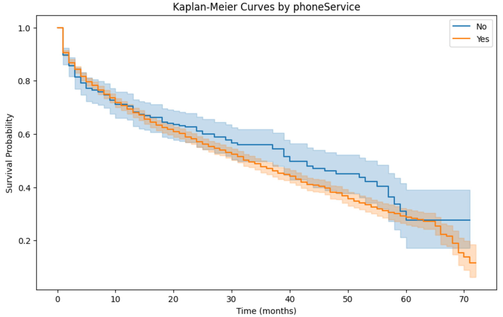Figure 6: Survival curve by phone service

---

1. Multiple Lines Service (multipleLines)

Group Comparison	test_statistic	p-value
No phone service vs No	12.382712	4.333273e-04
No vs Yes	72.358368	1.794602e-17
No phone service vs Yes	1.500291	0.2206266

• Conclusion: Multiple lines service has a significant impact on retention

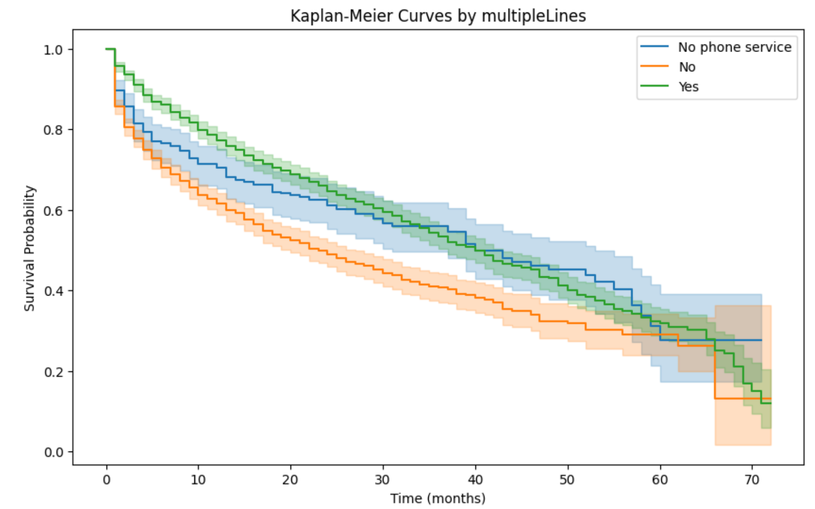Figure 7: Survival curve by multiple lines service

---

1. Internet Service Type (internetService)

Metric	Value
test_statistic	25.172866
p-value	5.241449e-07
-log2(p)	20.863531

• Conclusion: DSL customers retain significantly better than fiber optic customers

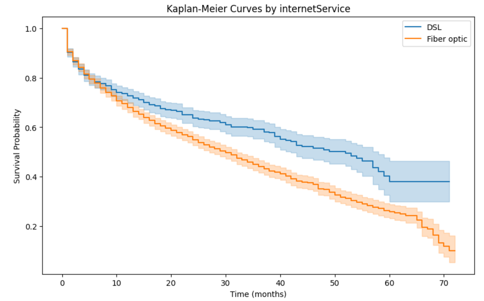Figure 8: Survival curve by internet service type

---

1. Streaming TV (streamingTV)

Metric	Value
test_statistic	12.93926
p-value	0.000322
-log2(p)	11.601718

• Conclusion: Customers with streaming TV service retain significantly better

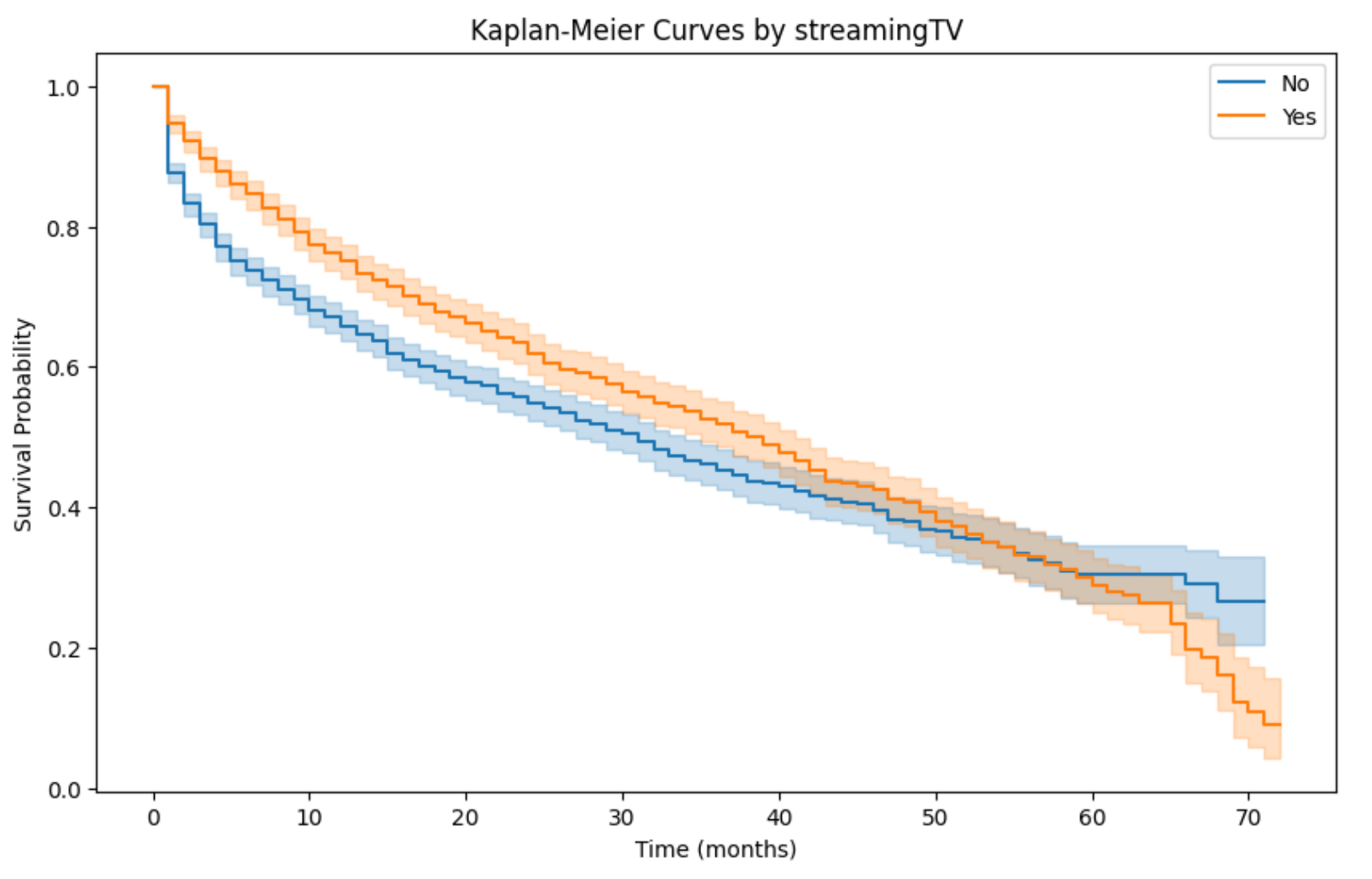Figure 9: Survival curve by streaming TV

---

1. Streaming Movies (streamingMovies)

Metric	Value
test_statistic	17.941685
p-value	0.000023
-log2(p)	15.422016

• Conclusion: Customers with streaming movies service retain significantly better

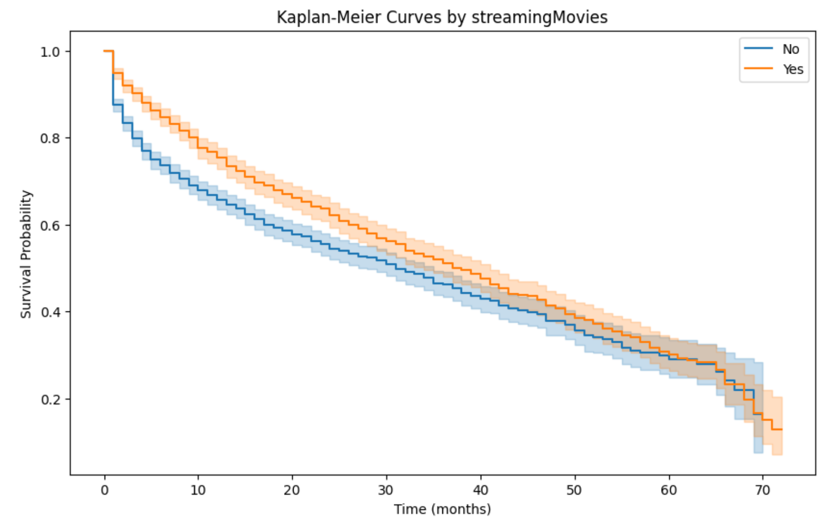Figure 10: Survival curve by streaming movies

---

1. Online Security Service (onlineSecurity)

Metric	Value
test_statistic	141.60316
p-value	1.187554e-32
-log2(p)	106.053706

• Conclusion: Customers with online security service have significantly longer retention time

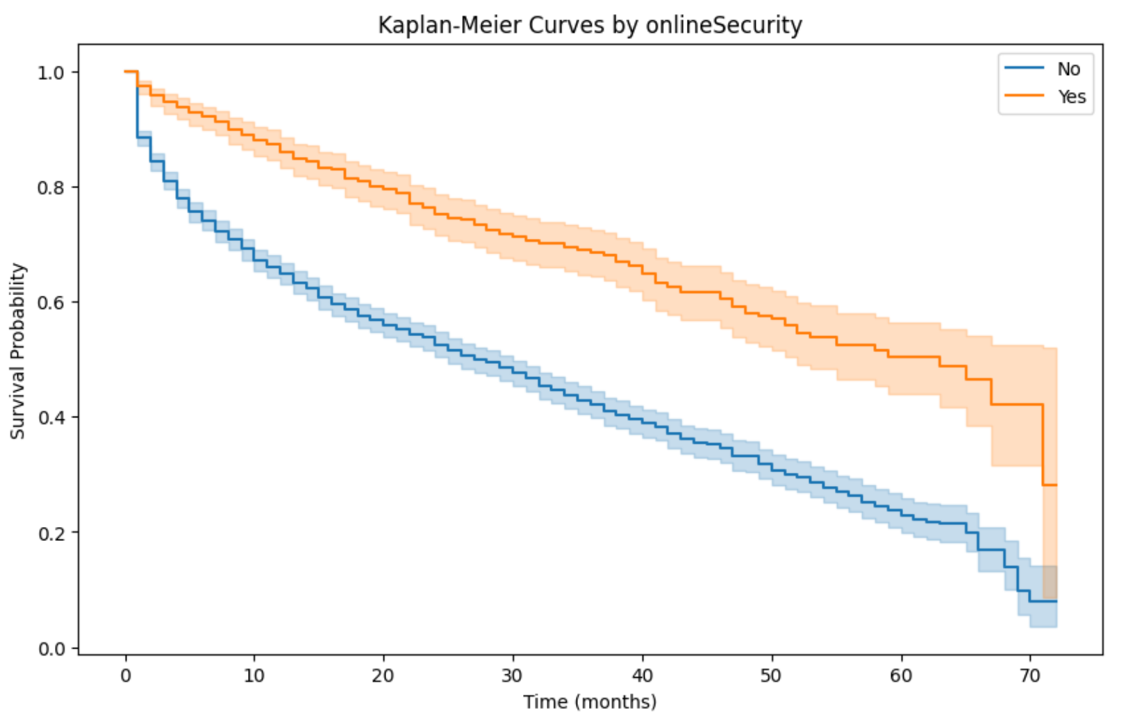Figure 11: Survival curve by online security

---

1. Online Backup Service (onlineBackup)

Metric	Value
test_statistic	189.482865
p-value	4.122979e-43
-log2(p)	140.799221

• Conclusion: Customers with online backup service have significantly longer retention time

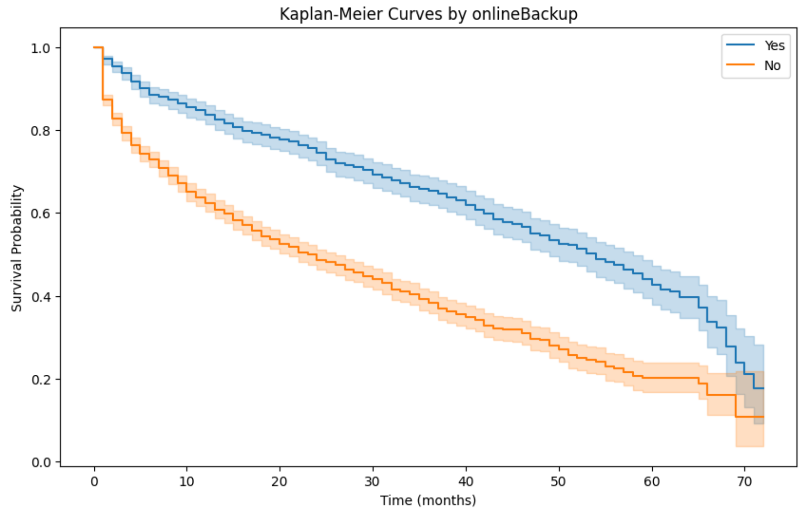Figure 12: Survival curve by online backup

---

1. Device Protection Service (deviceProtection)

Metric	Value
test_statistic	71.496825
p-value	2.777047e-17
-log2(p)	54.999226

• Conclusion: Customers with device protection service have significantly longer retention time

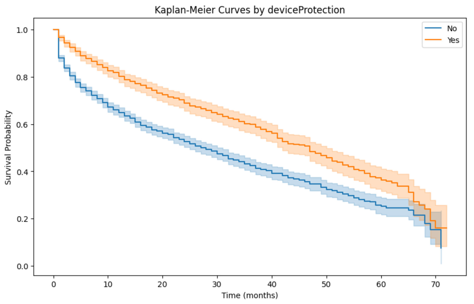Figure 13: Survival curve by device protection

---

1. Tech Support Service (techSupport)

Metric	Value
test_statistic	90.430334
p-value	1.916059e-21
-log2(p)	68.822348

• Conclusion: Customers with tech support service have significantly longer retention time

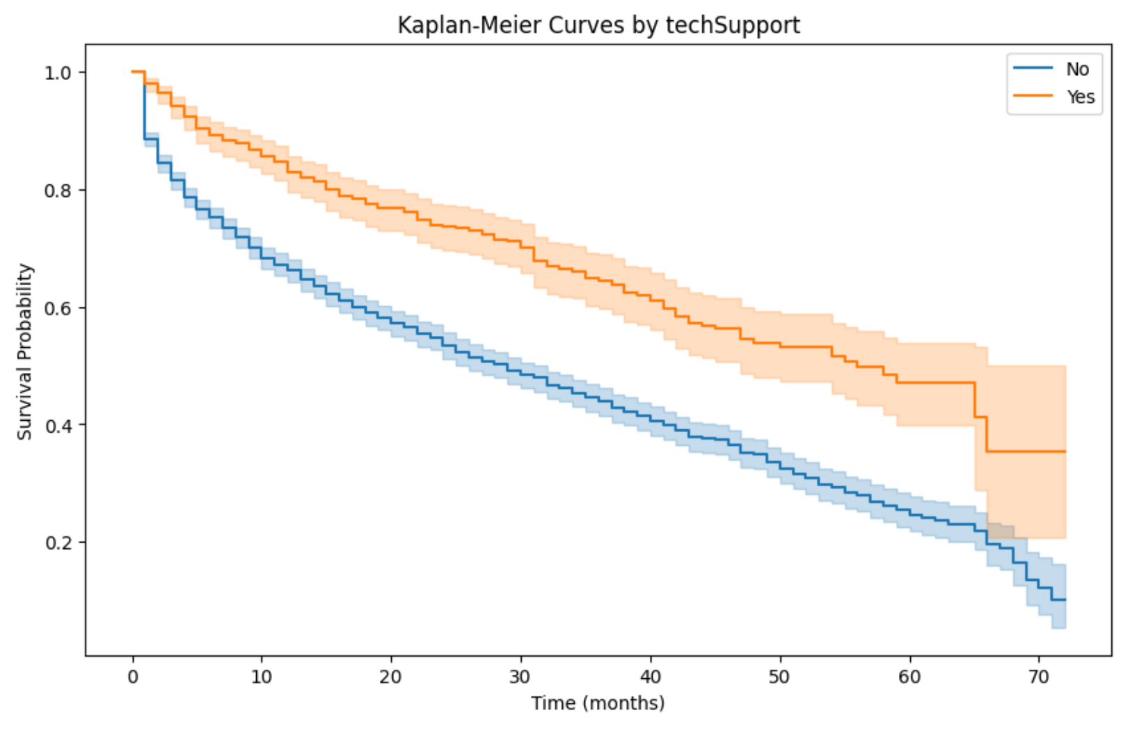Figure 14: Survival curve by tech support

---

1. Paperless Billing (paperlessBilling)

Metric	Value
test_statistic	8.340802
p-value	0.003876
-log2(p)	8.011049

• Conclusion: Customers using paperless billing have higher churn risk

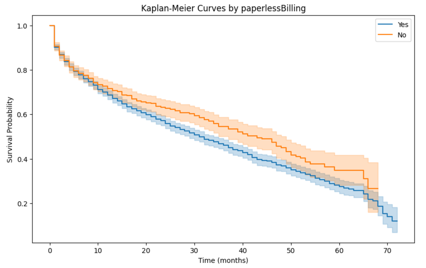Figure 15: Survival curve by paperless billing

---

1. Payment Method (paymentMethod)
   • Conclusion: Payment method has a highly significant impact on retention; electronic check is a high-risk payment method

Group Comparison	test_statistic	p-value	-log2(p)
Bank transfer (automatic) vs Credit card (automatic)	0.061543	8.040732e-01	0.314601
Bank transfer (automatic) vs Electronic check	91.191889	1.303937e-21	69.377616
Bank transfer (automatic) vs Mailed check	43.536998	4.160192e-11	34.484559
Credit card (automatic) vs Electronic check	79.991082	3.761035e-19	61.205504
Credit card (automatic) vs Mailed check	39.684613	2.984678e-10	31.641706
Electronic check vs Mailed check	0.898320	3.432326e-01	1.542741

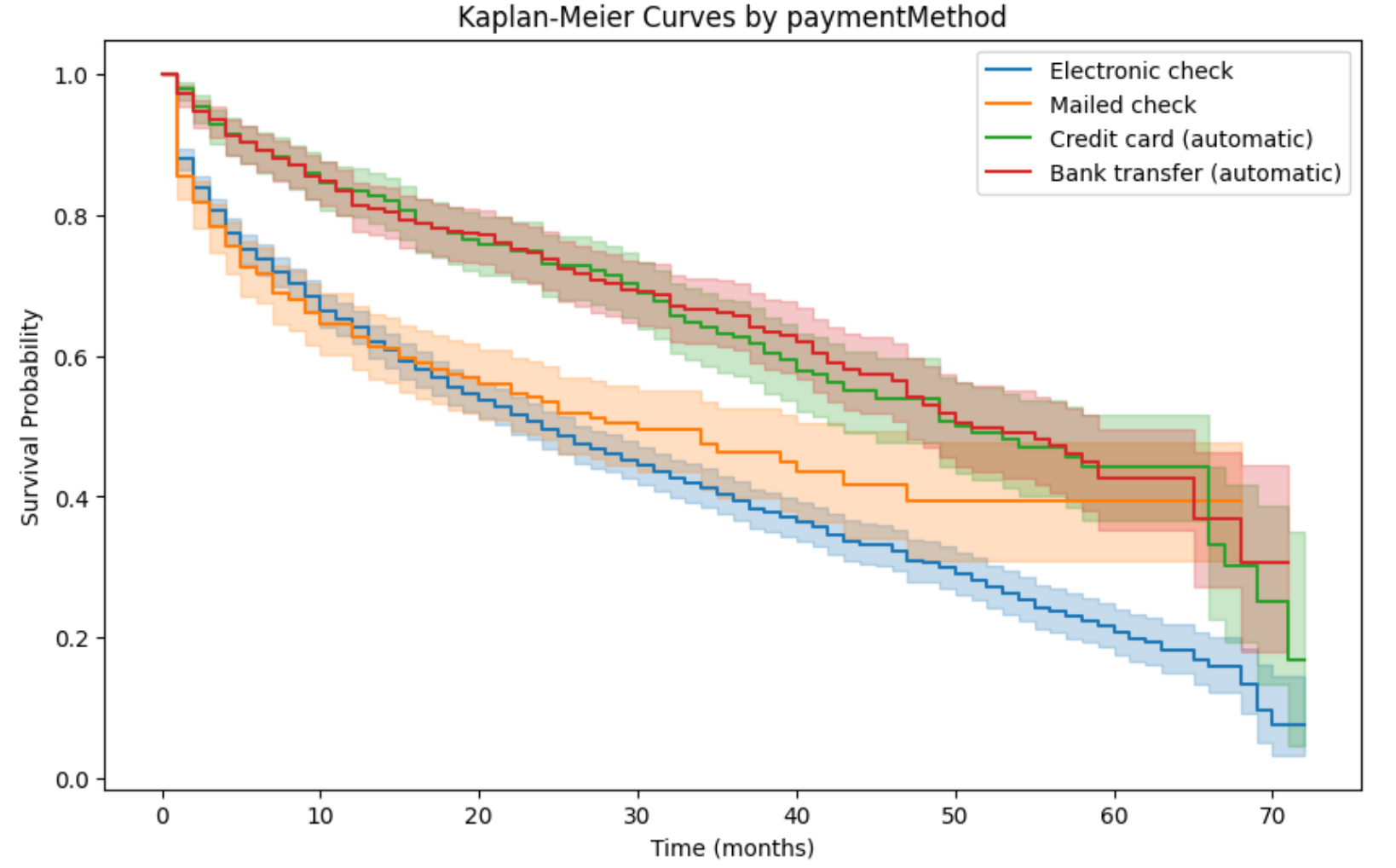Figure 16: Survival curve by payment method

4.2.4 Key Findings

1. Overall customer retention level
   The target customer segment has a median survival time of 34 months, meaning 50% of customers churn within 34 months of joining the network, indicating a relatively high overall churn risk.

2. Factors with no significant impact on retention
   Gender, senior citizen status, and phone service subscription do not significantly affect customer retention (p > 0.05).

3. Protective services that significantly extend customer retention
   Online backup, online security, tech support, and device protection all significantly reduce churn risk, with:
   • Online backup having the strongest effect (log-rank statistic as high as 189.48)
   • Online security second
   • Tech support also being a core protective factor
4. Service type differences
   • DSL customers retain significantly better than fiber optic customers; fiber optic customers are a key churn concern.
   • Customers with streaming TV and streaming movies have significantly better retention.

5. Impact of customer personal characteristics
   Customers with partners or dependents have lower churn risk; family-type customers are more stable.

6. Billing and payment method risk signals
   • Customers using paperless billing have higher churn risk.
   • Electronic check payment is the highest-risk payment method; automatic deductions (bank transfer/credit card) yield the best retention.
7. Summary of high-risk customer profile
   Customers without a partner, without dependents, using fiber optic internet service, not purchasing value-added services (security/backup/tech support/device protection), and paying by electronic check are the highest churn risk group in this analysis.

---

5. Cox Proportional Hazards Model

5.1 Analysis Workflow

from lifelines import CoxPHFitter

# Data preparation and One-Hot encoding
encode_cols = ['dependents', 'internetService', 'onlineBackup', 'techSupport', 'paperlessBilling']
encoded_pd = pd.get_dummies(telco_pd, columns=encode_cols, prefix=encode_cols, drop_first=False)

# Select variables
survival_pd = encoded_pd[['churn', 'tenure', 'dependents_Yes', 
                          'internetService_DSL', 'onlineBackup_Yes', 'techSupport_Yes']]

# Fit Cox model
cph = CoxPHFitter(alpha=0.05)
cph.fit(survival_pd, 'tenure', 'churn')

# Output results
cph.print_summary()
cph.plot(hazard_ratios=True)

# Proportional hazards assumption test
cph.check_assumptions(survival_pd, p_value_threshold=0.05)
cph.check_assumptions(survival_pd, p_value_threshold=0.05, show_plots=True)

5.2 Analysis Results

5.2.1 Model Overview

| Metric | Value | |——–|——-| | model | lifelines.CoxPHFitter | | duration col | tenure | | event col | churn | | baseline estimation | breslow | | number of observations | 3351 | | number of events observed | 1556 | | partial log-likelihood | -11315.95 | | Concordance | 0.64 | | Partial AIC | 22639.90 | | log-likelihood ratio test | 337.77 (df=4) | | -log2(p) of ll-ratio test | 236.24 |

5.2.2 Model Coefficients and Hazard Ratio Analysis

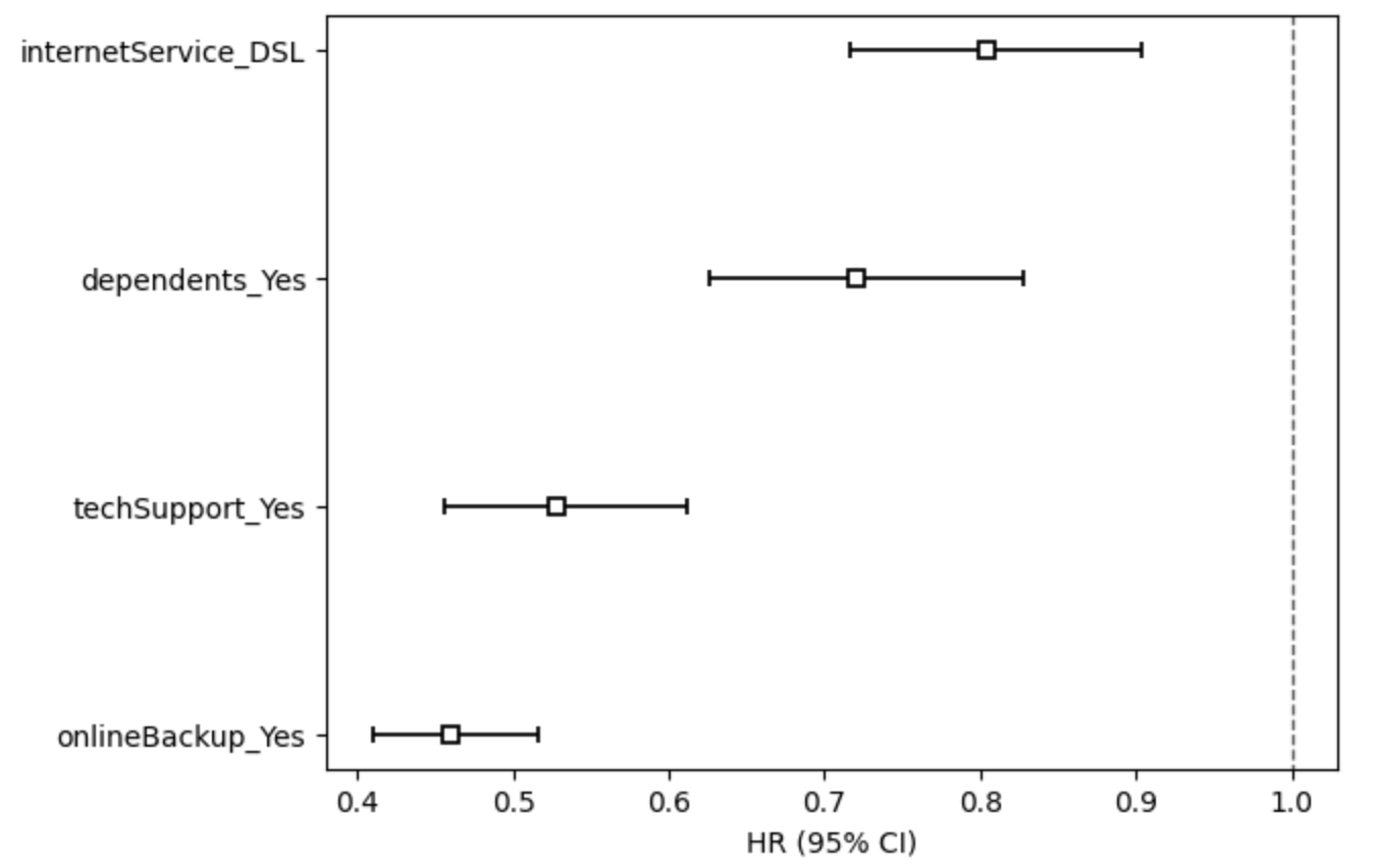Figure 17: Cox model hazard ratios (HR<1 indicates protective factor, with 95% CI)

Variable	coef	exp(coef)	se(coef)	coef 95% CI	exp(coef) 95% CI	z	p-value	-log2(p)	Significance
dependents_Yes	-0.33	0.72	0.07	[-0.47, -0.19]	[0.63, 0.83]	-4.64	<0.005	18.12	***
internetService_DSL	-0.22	0.80	0.06	[-0.33, -0.10]	[0.72, 0.90]	-3.68	<0.005	12.07	***
onlineBackup_Yes	-0.78	0.46	0.06	[-0.89, -0.66]	[0.41, 0.52]	-13.13	<0.005	128.37	***
techSupport_Yes	-0.64	0.53	0.08	[-0.79, -0.49]	[0.46, 0.61]	-8.48	<0.005	55.36	***

Significance markers: ** p<0.001, ** p<0.01, * p<0.05

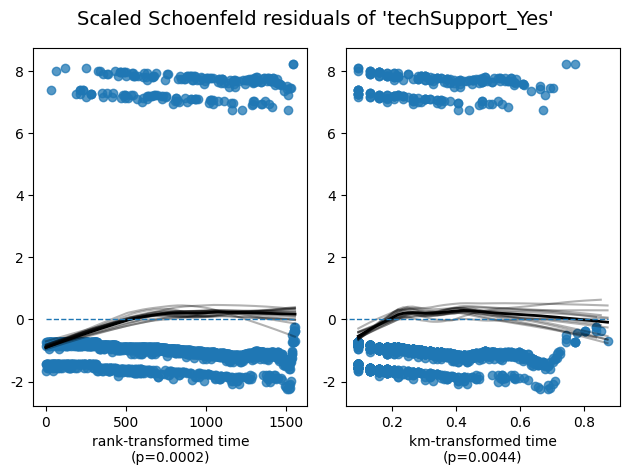
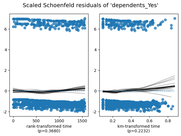
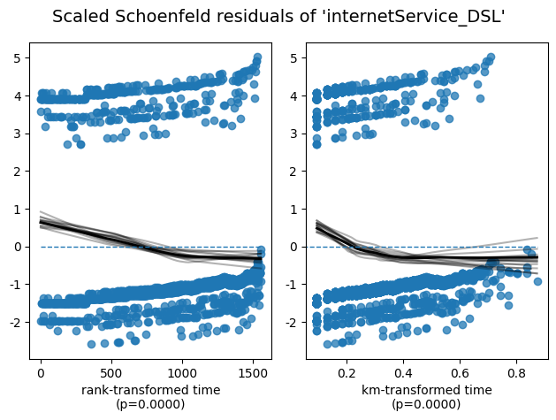
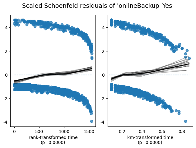
Figure 18: Scaled Schoenfeld residual plots for each variable (with both rank and km time transformation methods)

5.2.3 Proportional Hazards Assumption Test Results

Variable	Test Method	Test Statistic	p-value	-log2(p)	Assumption Check
dependents_Yes	km	1.48	0.22	2.16	Pass
dependents_Yes	rank	0.81	0.37	1.44	Pass
internetService_DSL	km	20.98	<0.005	17.72	Violated
internetService_DSL	rank	26.71	<0.005	22.01	Violated
onlineBackup_Yes	km	17.80	<0.005	15.31	Violated
onlineBackup_Yes	rank	17.47	<0.005	15.07	Violated
techSupport_Yes	km	8.09	<0.005	7.81	Violated
techSupport_Yes	rank	13.76	<0.005	12.23	Violated

The following variables violate the proportional hazards assumption:

1. internetService_DSL: p-value < 5e-05
2. onlineBackup_Yes: p-value < 5e-05
3. techSupport_Yes: p-value = 0.0002

Remedial suggestion: When modeling, use strata=['internetService_DSL', 'onlineBackup_Yes', 'techSupport_Yes'] to stratify variables that violate the assumption, improving model reliability.

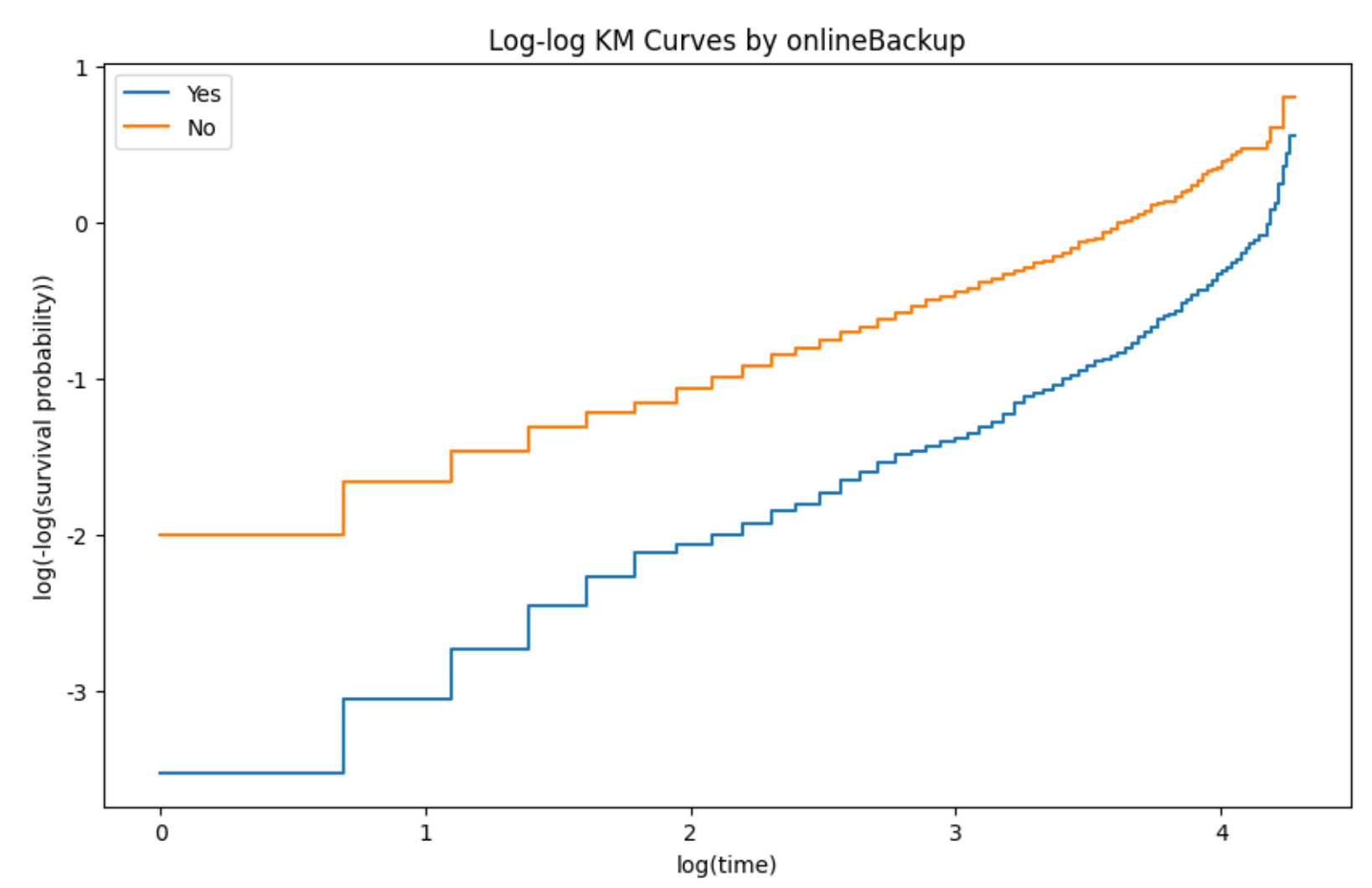
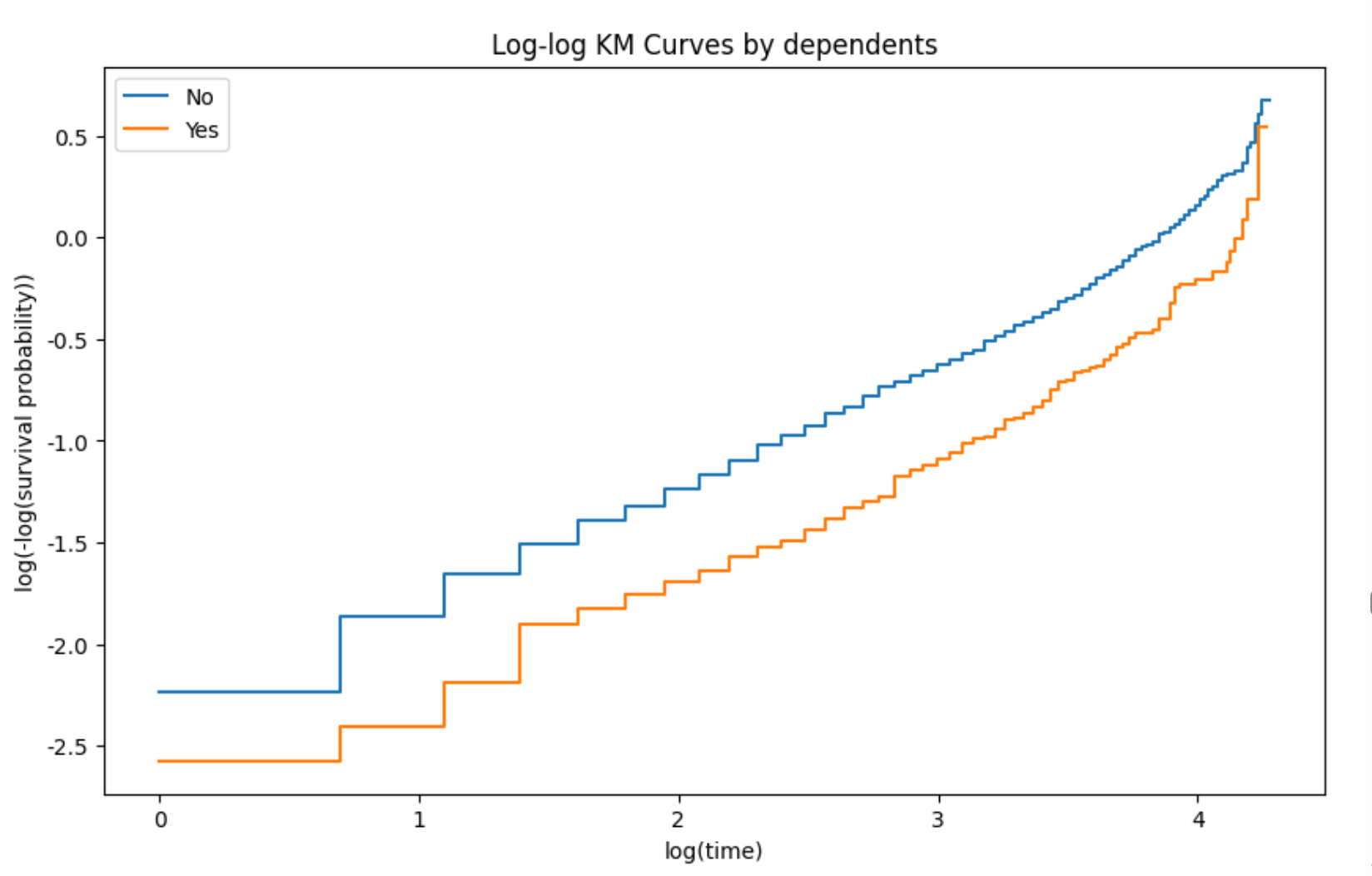
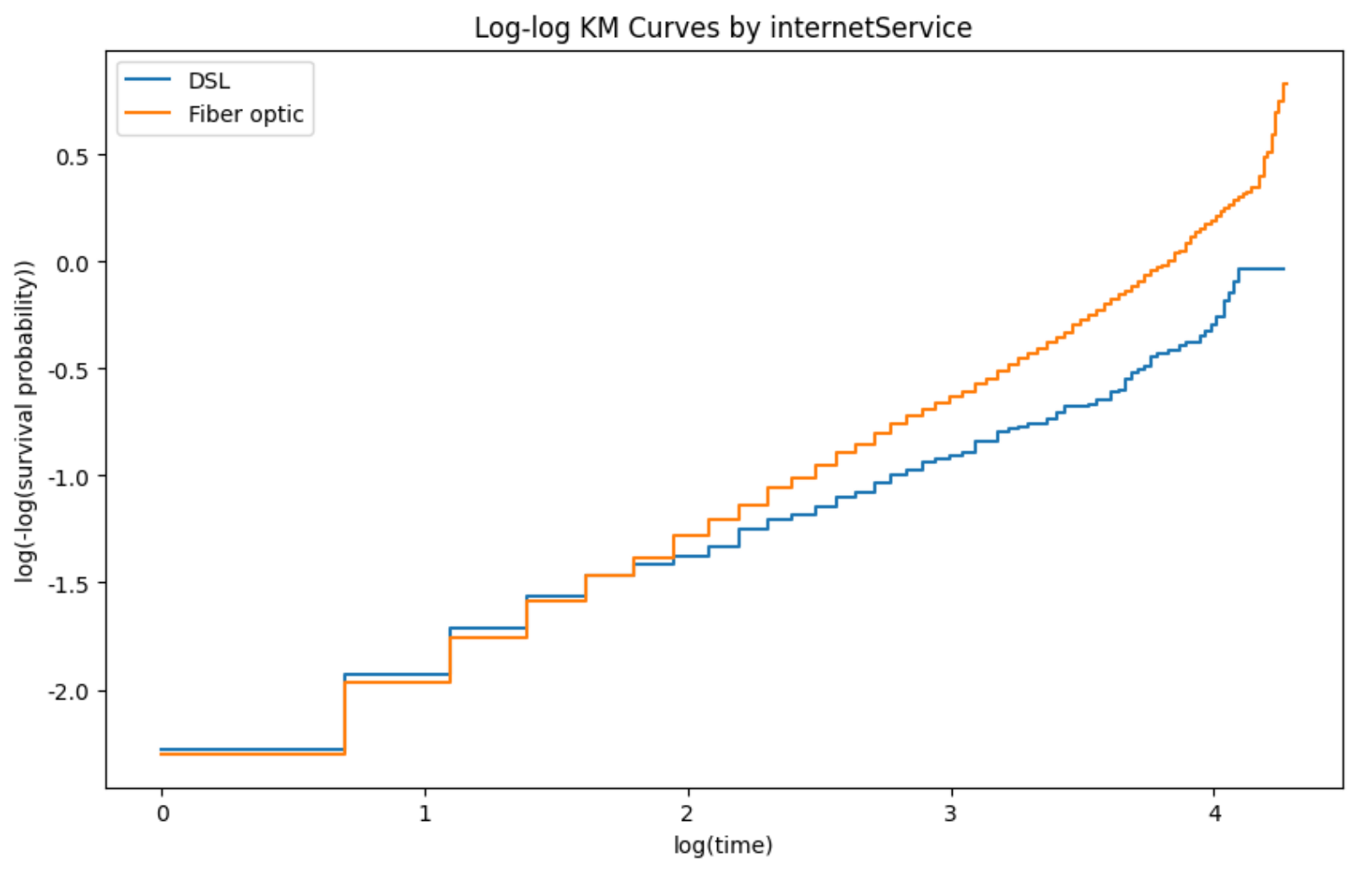
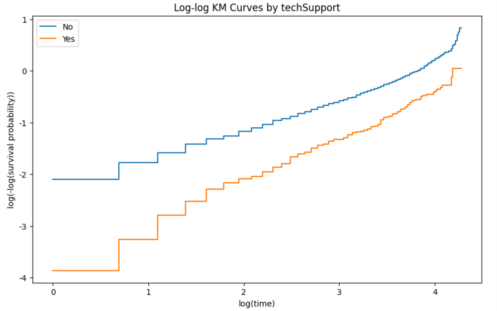
Figure 19: Log-log Kaplan-Meier curves for each variable group, used to visually verify the proportional hazards assumption

5.2.4 Key Findings

1. Protective factors (reducing customer churn risk)
   All variables included in this model are protective factors against customer churn, ordered by effect strength as follows:
   • onlineBackup_Yes: HR=0.46, reduces customer churn risk by 54.0% (p<0.001) – strongest churn inhibition factor
   • techSupport_Yes: HR=0.53, reduces customer churn risk by 47.2% (p<0.001)
   • dependents_Yes: HR=0.72, reduces customer churn risk by 28.0% (p<0.001)
   • internetService_DSL: HR=0.80, reduces customer churn risk by 19.5% (p<0.001)
2. Risk factors
   In the Cox regression model constructed in this study, no risk factors with HR>1.2 and statistical significance were identified. All included features showed a positive effect on customer retention.

---

6. Accelerated Failure Time Model (AFT)

6.1 Analysis Workflow

from lifelines import LogLogisticAFTFitter

# Data preparation and One-Hot encoding
encode_cols = ['partner', 'multipleLines', 'internetService', 'onlineSecurity', 
               'onlineBackup', 'deviceProtection', 'techSupport', 'paymentMethod']
encoded_pd = pd.get_dummies(telco_pd, columns=encode_cols, prefix=encode_cols, drop_first=False)

# Select variables
survival_pd = encoded_pd[['churn', 'tenure', 'partner_Yes', 'multipleLines_Yes',
                          'internetService_DSL', 'onlineSecurity_Yes', 'onlineBackup_Yes',
                          'deviceProtection_Yes', 'techSupport_Yes',
                          'paymentMethod_Bank transfer (automatic)',
                          'paymentMethod_Credit card (automatic)']]

# Fit LogLogistic AFT model
aft = LogLogisticAFTFitter()
aft.fit(survival_pd, duration_col='tenure', event_col='churn')

# Output results
print(f"Median Survival Time:{np.exp(aft.median_survival_time_):.2f}")
aft.print_summary()
aft.plot()

6.2 Analysis Results

6.2.1 Model Results

Metric	Value
model	lifelines.LogLogisticAFTFitter
duration col	tenure
event col	churn
baseline estimation	breslow
number of observations	3351
number of events observed	1556
log-likelihood	-6838.36
Concordance	0.73
AIC	13698.72
log-likelihood ratio test	877.49 (df=9)
-log2(p) of ll-ratio test	605.78

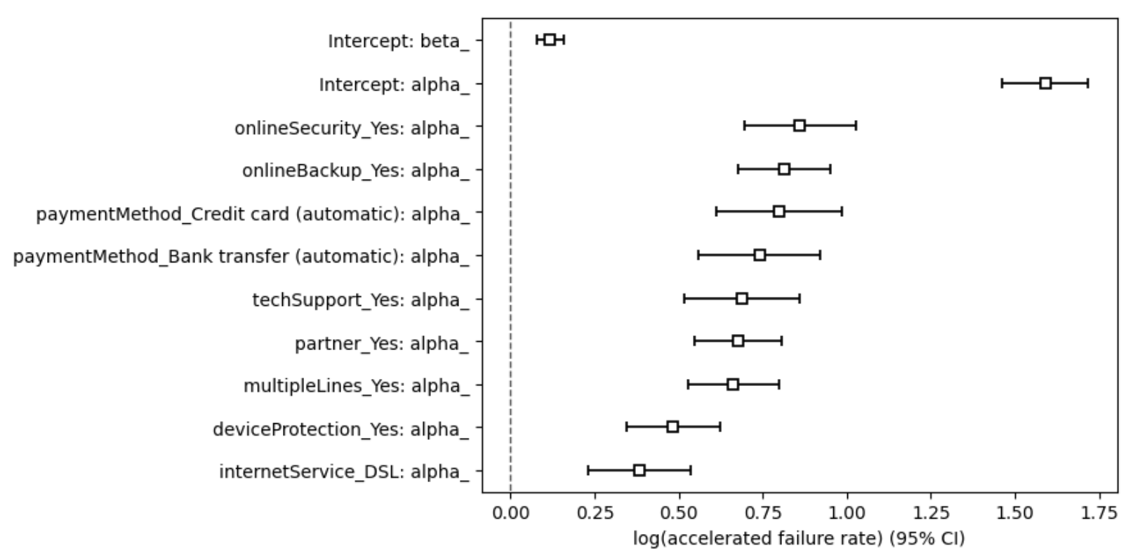Figure 20: AFT model coefficients and confidence intervals

6.2.2 AFT Model Coefficient Table

Variable	coef	exp(coef)	se(coef)	z	p	-log2(p)
deviceProtection_Yes	0.48	1.62	0.07	6.88	<0.005	-
internetService_DSL	0.38	1.47	0.08	4.98	<0.005	-
multipleLines_Yes	0.66	1.94	0.07	9.64	<0.005	-
onlineBackup_Yes	0.81	2.25	0.07	11.63	<0.005	-
onlineSecurity_Yes	0.86	2.37	0.09	10.12	<0.005	-
partner_Yes	0.68	1.97	0.07	10.21	<0.005	-
paymentMethod_Bank transfer	0.74	2.10	0.09	8.05	<0.005	-
paymentMethod_Credit card	0.80	2.22	0.10	8.36	<0.005	-
techSupport_Yes	0.69	1.99	0.09	7.90	<0.005	-
Intercept	1.59	4.91	0.07	24.47	<0.005	-
beta_Intercept	0.12	1.13	0.02	5.71	<0.005	-

6.2.3 Model Assumption Verification - Log-odds Plots

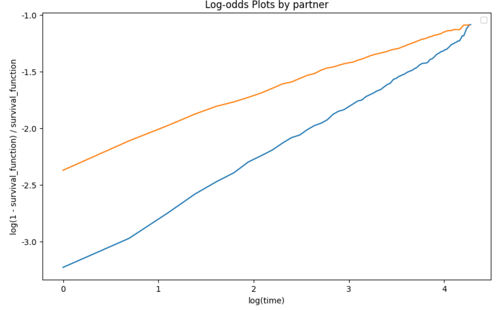Figure 21: Log-odds plot (partner)

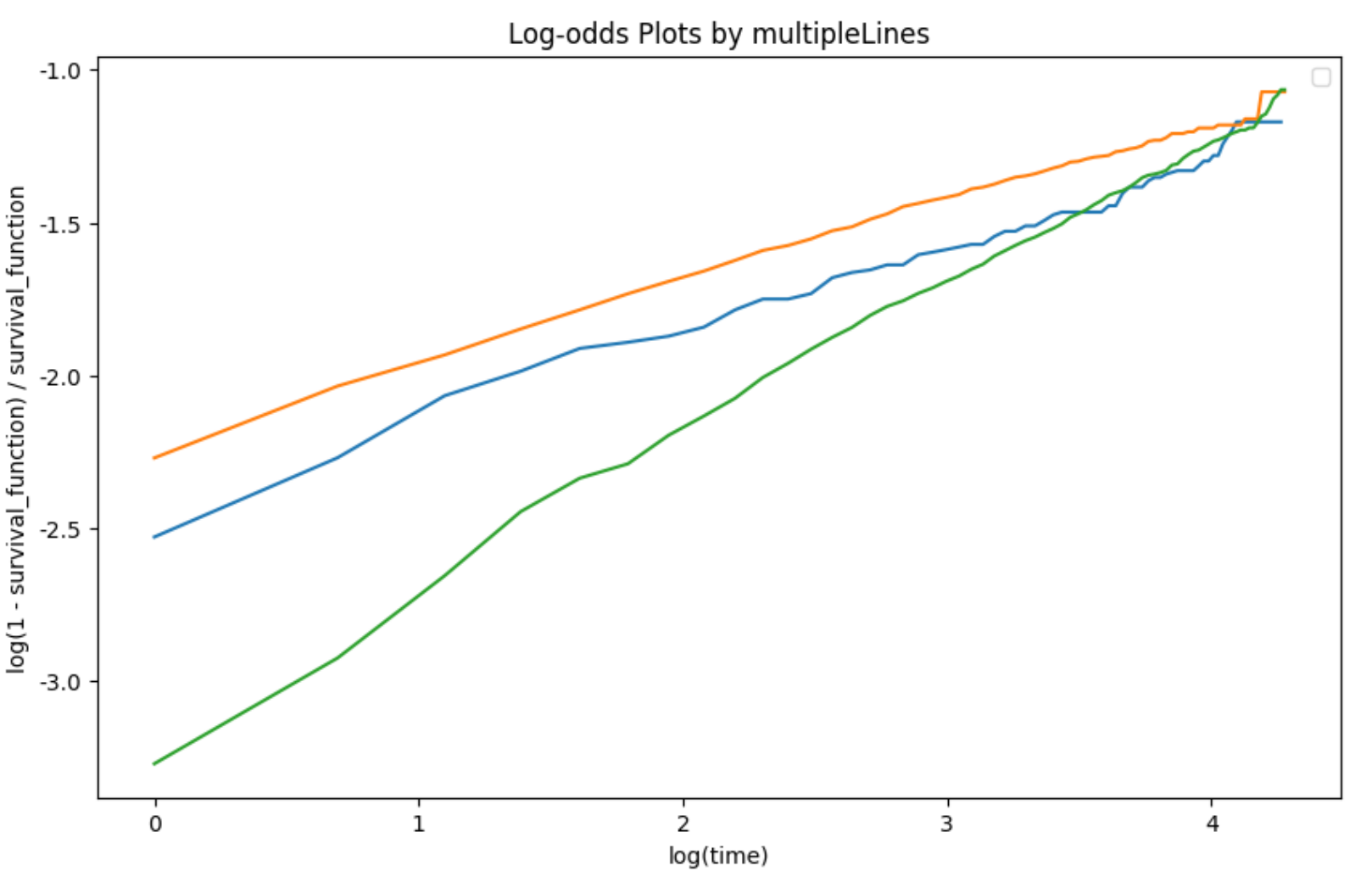Figure 22: Log-odds plot (multipleLines)

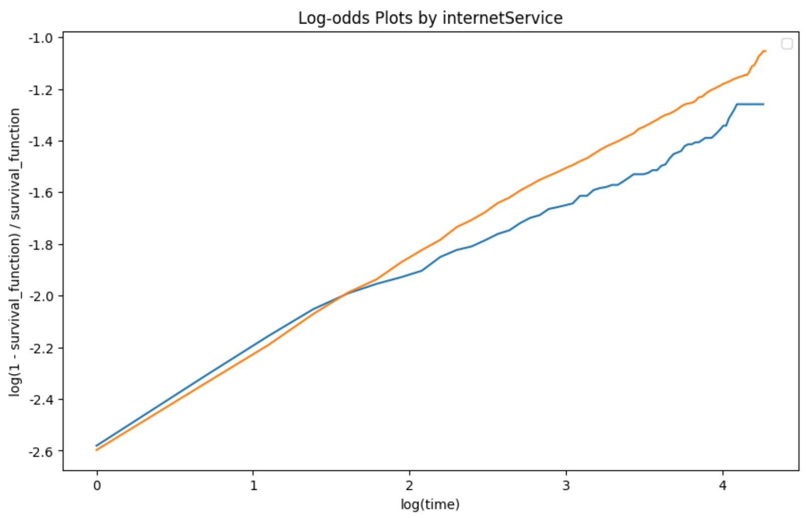Figure 23: Log-odds plot (internetService)

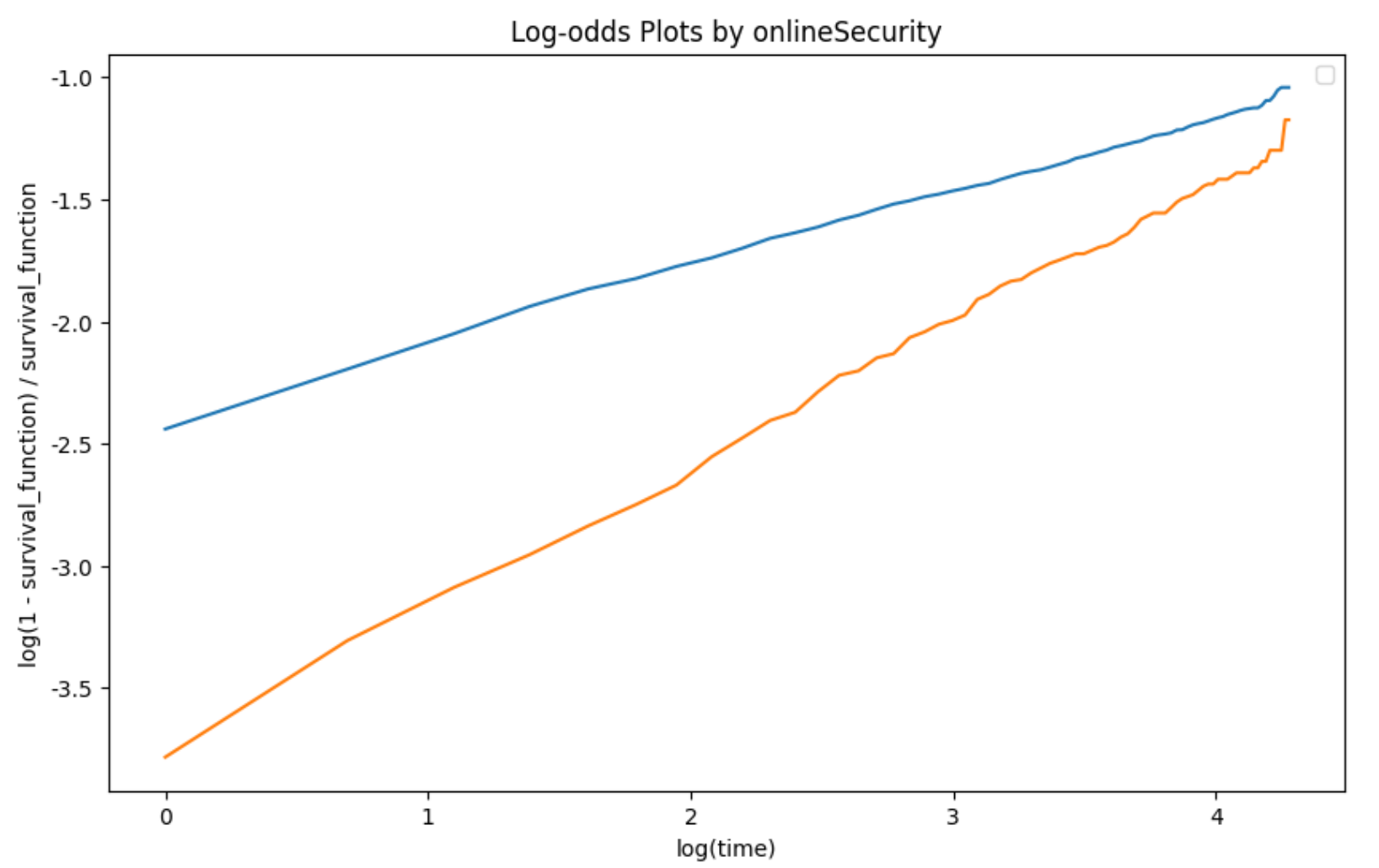Figure 24: Log-odds plot (onlineSecurity)

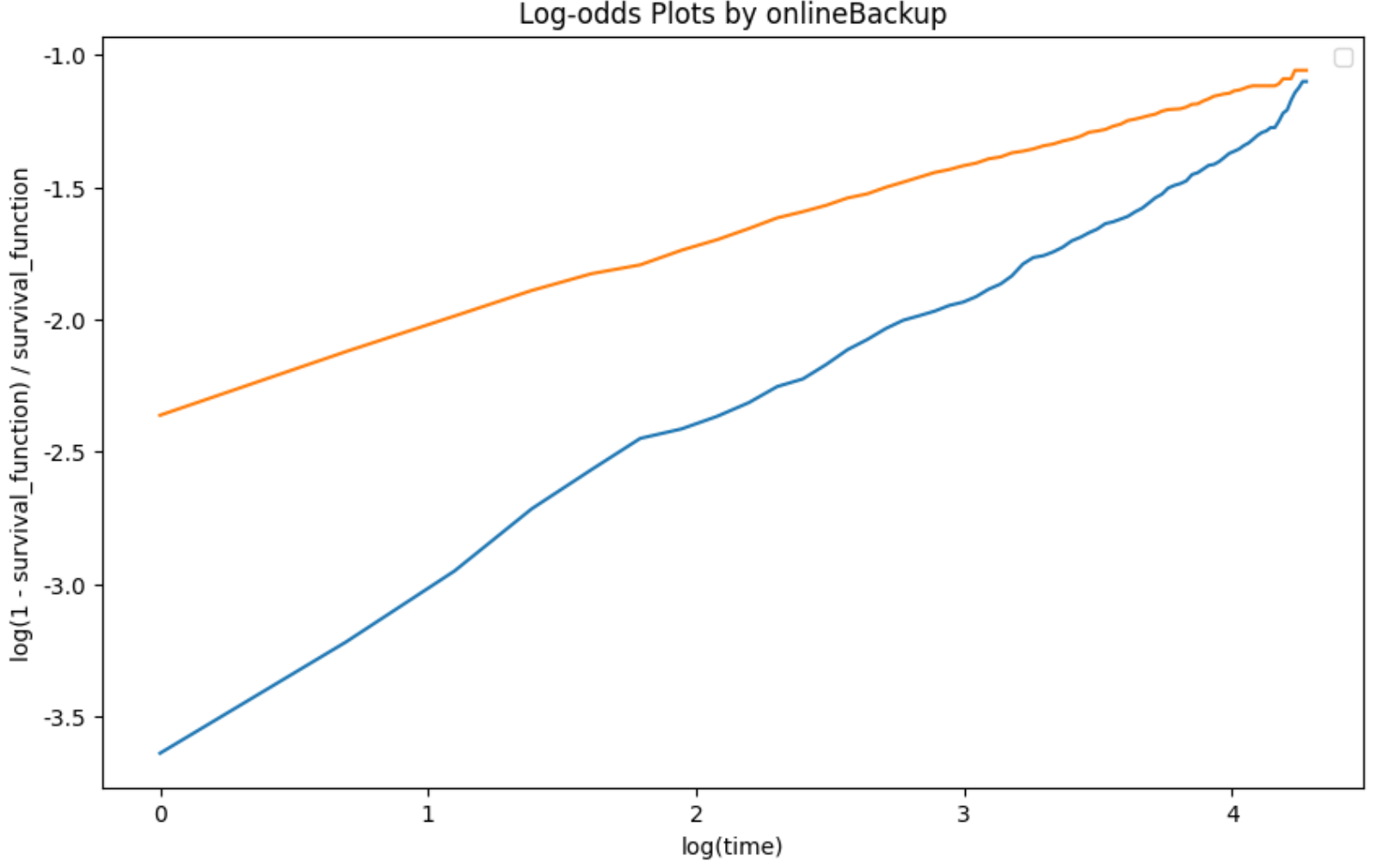Figure 25: Log-odds plot (onlineBackup)

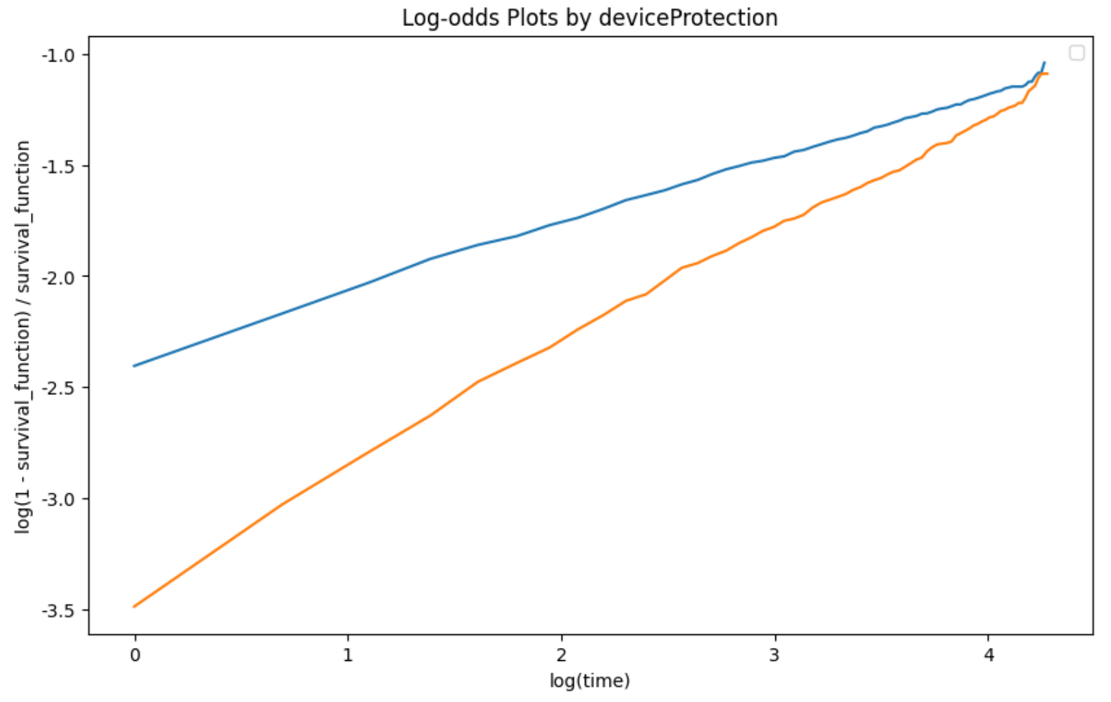Figure 26: Log-odds plot (deviceProtection)

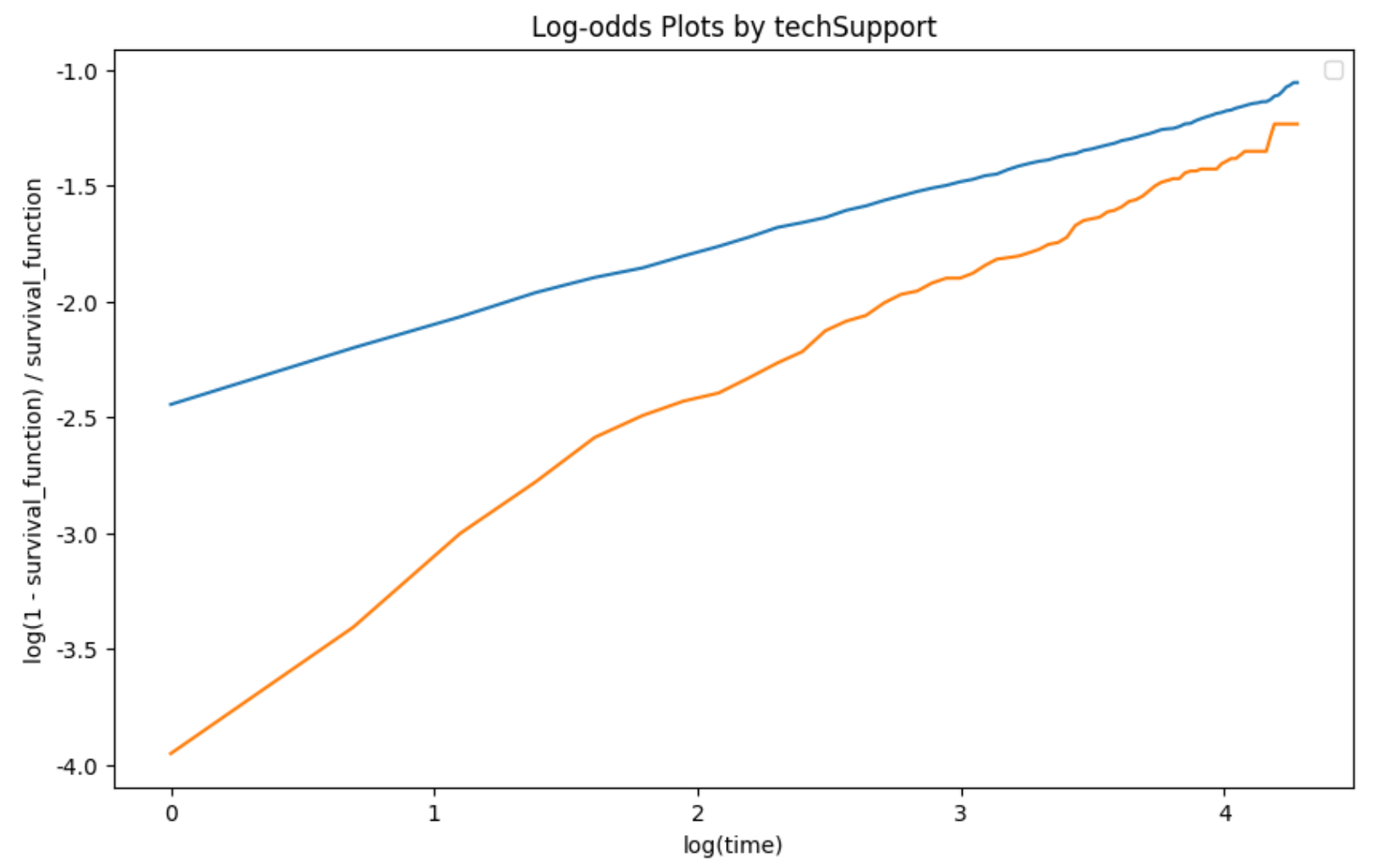Figure 27: Log-odds plot (techSupport)

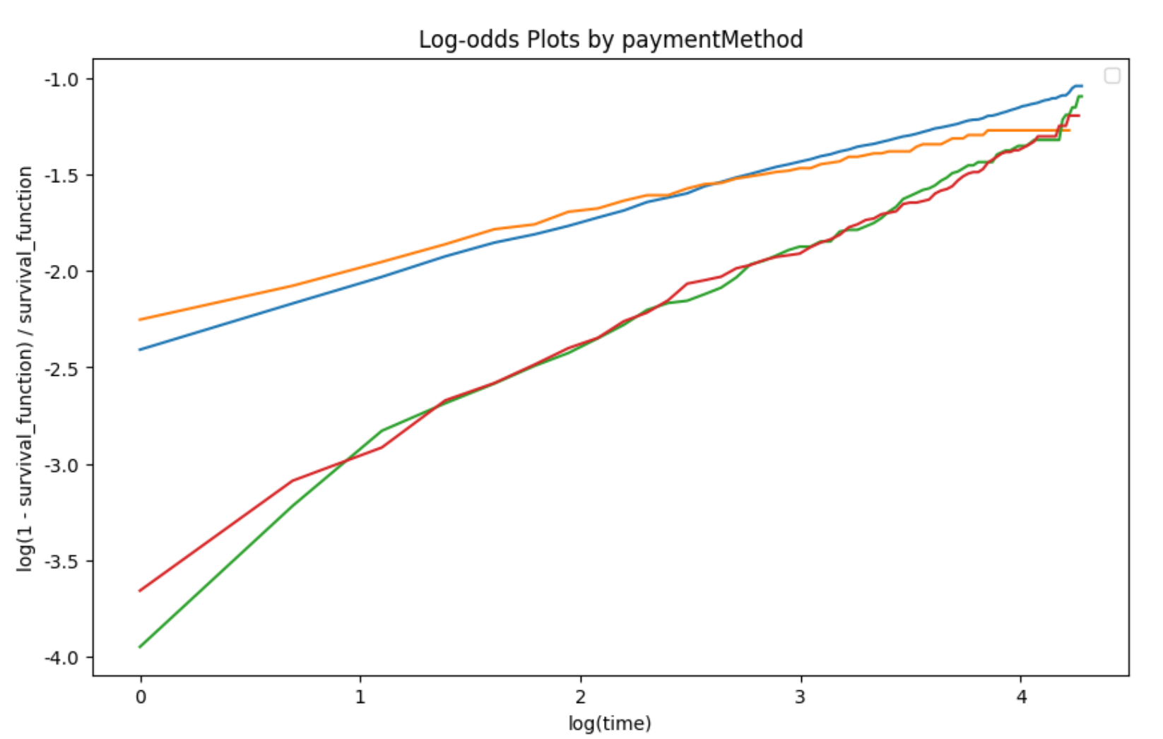Figure 28: Log-odds plot (paymentMethod)

6.2.4 Reliability Warnings

• Warning 1: Predicted value (135.5) exceeds 1.5 times the data range (72.0)
• Warning 2: Large discrepancy from Kaplan-Meier result (34.0), ratio = 3.99

6.2.5 Recommendation

Do not use AFT model results for business decisions. Use Kaplan-Meier results (34 months) instead.

---

7. Customer Lifetime Value (CLV)

7.1 Calculation Workflow

def calculate_customer_lifetime_value(cph, monthly_profit=30, discount_rate=0.10):
    # Define baseline customer
    baseline_customer = pd.DataFrame([{
        'dependents_Yes': 0, 'internetService_DSL': 0,
        'onlineBackup_Yes': 0, 'techSupport_Yes': 0
    }])
    
    irr = discount_rate / 12
    survival_func = cph.predict_survival_function(baseline_customer)
    
    # Build cohort table
    cohort_df = pd.concat([pd.DataFrame([1.00]), round(survival_func, 2)])
    cohort_df = cohort_df.rename(columns={0: 'Survival Probability'})
    cohort_df['Contract Month'] = cohort_df.index.astype('int')
    cohort_df['Monthly Profit for the Selected Plan'] = monthly_profit
    cohort_df['Avg Expected Monthly Profit'] = round(cohort_df['Survival Probability'] * monthly_profit, 2)
    cohort_df['NPV of Avg Expected Monthly Profit'] = round(
        cohort_df['Avg Expected Monthly Profit'] / ((1 + irr) ** cohort_df['Contract Month']), 2
    )
    cohort_df['Cumulative NPV'] = cohort_df['NPV of Avg Expected Monthly Profit'].cumsum()
    cohort_df['Contract Month'] = cohort_df['Contract Month'] + 1
    
    return cohort_df.set_index('Contract Month')

7.2 Calculation Results

7.2.1 Calculation Parameters

• Monthly profit per customer: $30
• Annual discount rate: 10%
• Monthly discount rate: 0.83%
• Forecast time horizon: 72 months

7.2.2 CLV Key Node Results

Time Horizon	Cumulative NPV (CLV)
12 months	$266.88
24 months	$405.44
36 months	$515.01
Lifetime CLV	$626.69

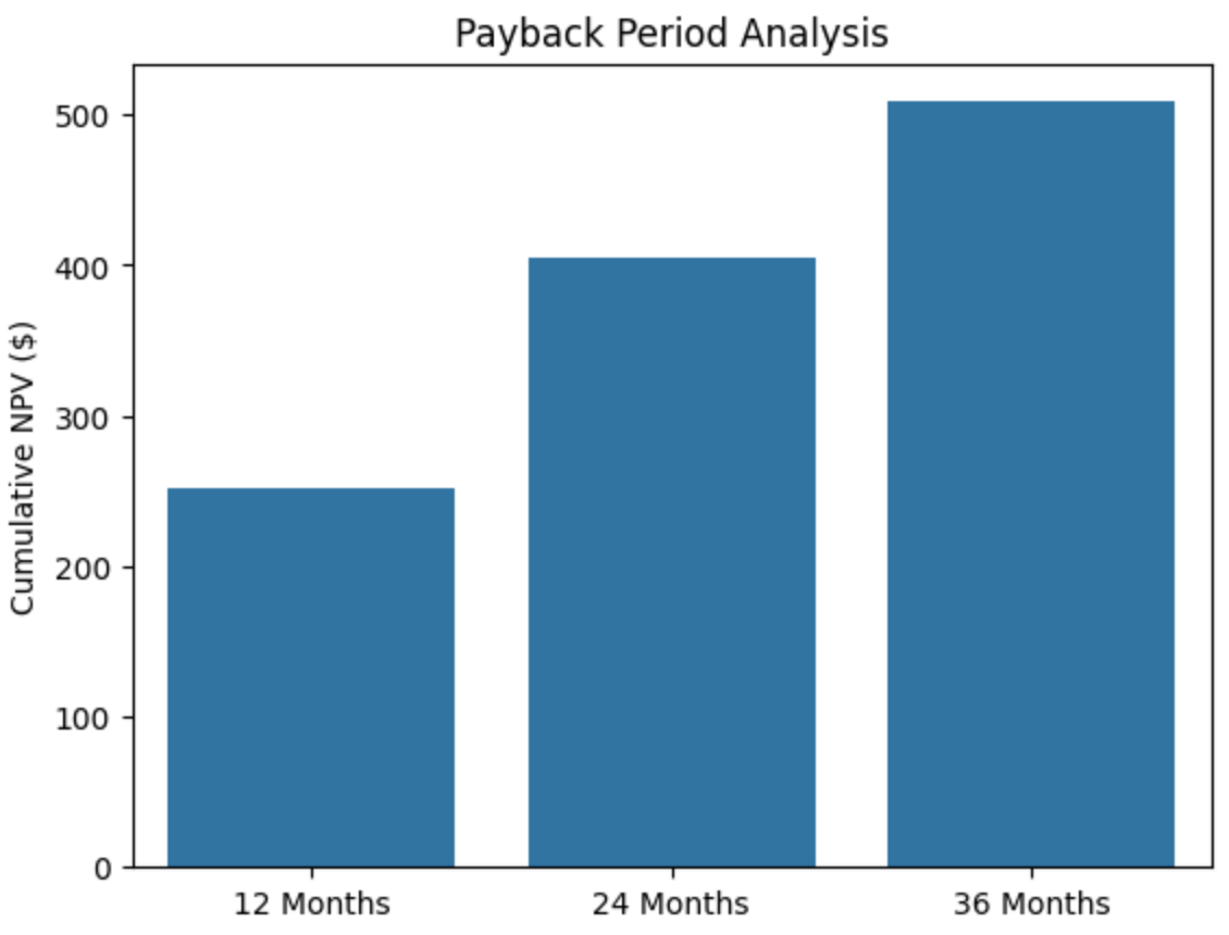Figure 29: Payback period analysis

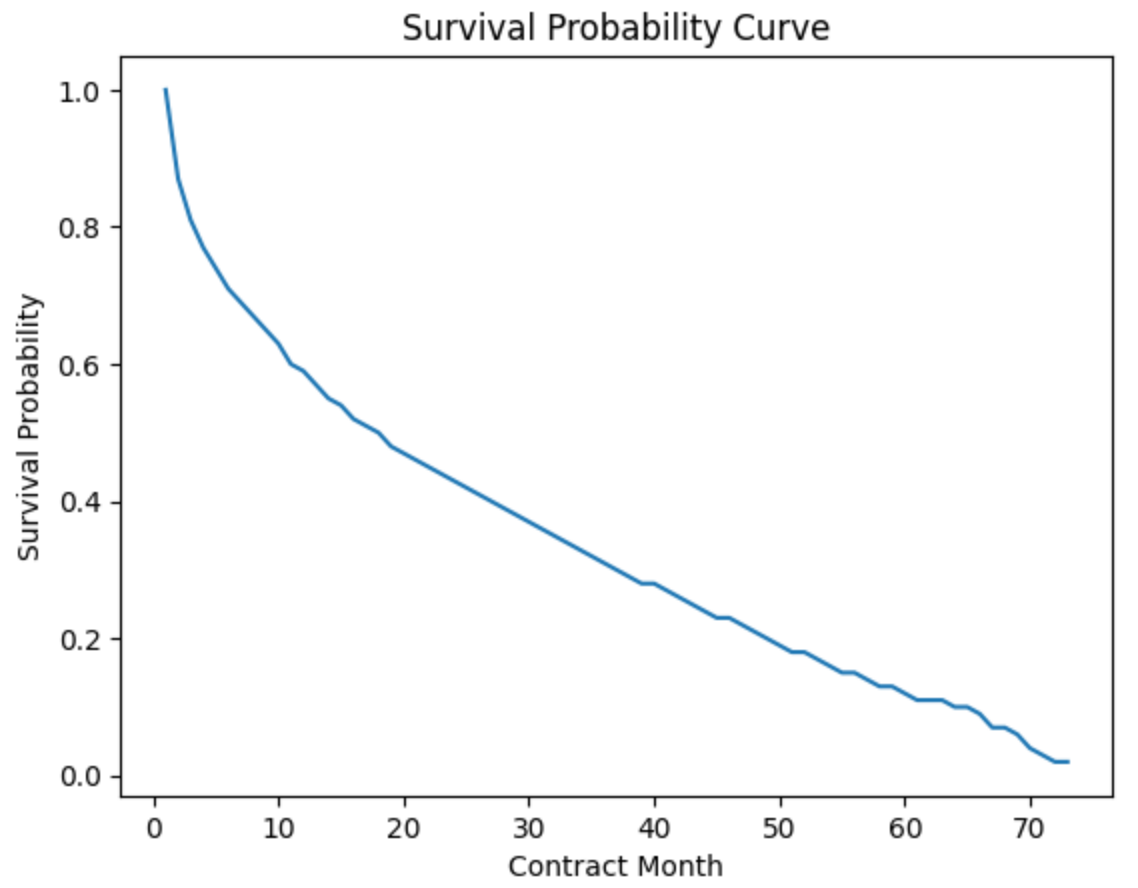Figure 30: Survival probability curve

7.2.3 CLV Trend Table (complete data for first 25 months)

Contract Month	Survival Probability	Monthly Profit	Avg Expected Monthly Profit	NPV	Cumulative NPV
1	1.00	30	30.00	30.00	30.00
2	0.87	30	26.10	25.88	55.88
3	0.81	30	24.30	23.90	79.78
4	0.77	30	23.10	22.53	102.31
5	0.74	30	22.20	21.48	123.79
6	0.71	30	21.30	20.43	144.22
7	0.69	30	20.70	19.69	163.91
8	0.67	30	20.10	18.97	182.88
9	0.65	30	19.50	18.25	201.13
10	0.63	30	18.90	17.54	218.67
11	0.60	30	18.00	16.57	235.24
12	0.59	30	17.70	16.16	251.40
13	0.57	30	17.10	15.48	266.88
14	0.55	30	16.50	14.81	281.69
15	0.54	30	16.20	14.42	296.11
16	0.52	30	15.60	13.77	309.88
17	0.51	30	15.30	13.40	323.28
18	0.50	30	15.00	13.03	336.31
19	0.48	30	14.40	12.40	348.71
20	0.47	30	14.10	12.04	360.75
21	0.46	30	13.80	11.69	372.44
22	0.45	30	13.50	11.34	383.78
23	0.44	30	13.20	11.00	394.78
24	0.43	30	12.90	10.66	405.44
25	0.42	30	12.60	10.32	415.76

7.2.4 Key Findings

1. Customer Lifetime Value (CLV): The cumulative net present value (NPV) for the baseline customer over 72 months is $626.69, a core reference metric for setting customer acquisition cost limits.
2. Revenue growth trend: Customer CLV grows rapidly to $266.88 in the first 12 months, to $405.44 by 24 months, and reaches $515.01 by 36 months, then growth slows, indicating the early period is critical for value contribution.
3. Survival probability decay: Customer survival probability continuously declines over time, from 1.00 in the first month to 0.43 by 24 months, reflecting the long-term trend of customer churn.
4. Impact of expected profit and discounting: Due to decaying survival probability and the discount rate, the average expected monthly profit per customer gradually declines from $30.00 in the first month to $12.90 by 24 months, and the growth rate of NPV also slows.
5. Business decision recommendations: Customer acquisition cost (CAC) should be controlled within 30% of CLV (approximately $188) to ensure profitability of customer relationships; at the same time, focus on implementing customer retention strategies within the first 24 months to maximize long-term customer value.

---

8. Conclusion

8.1 Model Applicability and Reliability Assessment

Based on the IBM Telco Customer Churn dataset, this study systematically quantifies churn behavior of month-to-month internet service customers using Kaplan-Meier estimation, Cox proportional hazards regression, Accelerated Failure Time (AFT) models, and the Customer Lifetime Value (CLV) framework. Main model evaluation conclusions are as follows:

Model	Reliability	Primary Use	Key Output
Kaplan-Meier estimation	✅ Highly reliable	Non-parametric survival function estimation	Median survival time: 34 months
Cox proportional hazards model	✅ Reliable	Multi-factor hazard ratio analysis	Concordance Index: 0.64; HR(onlineBackup)=0.46
LogLogistic AFT model	❌ Unreliable	Parametric survival time prediction	Predicted median survival time 135.5 months (beyond observation range)
CLV framework	✅ Usable	Long-term customer value quantification	72-month cumulative NPV: $626.69

Overall judgment: The Kaplan-Meier and Cox models provide robust core analytical conclusions for this study; the AFT model is not suitable for business decisions due to extrapolation beyond supported data range; the CLV framework, while informative, depends on the predictive ability of the Cox model.

8.2 Core Empirical Findings

(1) Overall customer retention level

The target customer segment (month-to-month + internet service users) has a median survival time of 34 months. This indicates that 50% of customers in this segment churn within 34 months after joining the network, representing a relatively high overall churn risk.

(2) Identification of key protective factors (based on Cox model)

Four variables were identified as significant protective factors, ordered by effect strength:

Protective Factor	Hazard Ratio (HR)	Reduction in Churn Risk	Statistical Significance
onlineBackup_Yes	0.46	54.0%	p < 0.001
techSupport_Yes	0.53	47.2%	p < 0.001
dependents_Yes	0.72	28.0%	p < 0.001
internetService_DSL	0.80	19.5%	p < 0.001

These results indicate that online backup and tech support services are the two most effective interventions for reducing customer churn risk. The Cox model’s Concordance Index is 0.64, indicating moderate discriminative ability.

(3) High-risk customer profile

Combining KM group analysis and marginal effects from the Cox model, high-risk churn customers exhibit the following typical characteristics:

• Demographic characteristics: No partner, no dependents
• Service usage characteristics: Use fiber optic internet service, not subscribed to value-added services such as online backup/online security/device protection/tech support
• Payment behavior characteristics: Pay by electronic check, use paperless billing

Log-rank test results show that the between-group difference for partner status is 135.76 (p < 2.25e-31), for dependents is 35.03 (p < 3.24e-09), and for fiber vs. DSL users is 25.17 (p < 5.24e-07), all statistically significant.

(4) Customer Lifetime Value (CLV)

The 72-month cumulative NPV for the baseline customer (not subscribed to any value-added services) predicted by the Cox model is $626.69. Of this, the first 12 months contribute $266.88 (42.6% of total value), and the first 24 months contribute $405.44 (64.7% of total value), indicating that customer value is concentrated in the first two years after joining.

8.3 Summary of Methodological Limitations

• Unreliability of the AFT model: The LogLogistic AFT model predicted a median survival time (135.5 months) significantly exceeding the actual observed range (0–72 months), with a ratio of 3.99 compared to the KM estimate (34 months). This deviation arises from the combination of high censoring rate and insufficient observation window, limiting the model’s extrapolation ability.
• Partial violation of proportional hazards assumption: In the Cox model, the variables internetService_DSL, onlineBackup_Yes, and techSupport_Yes did not pass the proportional hazards test (p < 0.05), suggesting that the effects of these variables may change over time. Stratified Cox or time-varying covariate models are recommended to address this.
• Sample selection bias: This study includes only month-to-month contract customers who subscribe to internet services. Conclusions cannot be directly generalized to long-term contract customers or those without internet service.

---

9. Business Recommendations

9.1 Short-term Operational Strategies (0–6 months)

(1) Value-added service promotion plan

Based on the hazard ratio estimates from the Cox model, online backup (HR=0.46) and tech support (HR=0.53) are the most effective risk mitigation tools. Recommendations:

• Implement bundling strategies for new customers, offering online backup and tech support as default add-ons to internet service with a first-month free trial.
• Conduct targeted marketing campaigns for existing high-risk customers (fiber users, those without partners/dependents) via email, in-app notifications, etc., to promote these services.
• Establish an A/B testing framework to quantify the causal effect of interventions on retention.

(2) Early identification of high-risk customers

Based on median survival time differences from KM group analysis:

Risk Dimension	High-risk Group	Low-risk Group	Median Survival Time Difference
Partner status	No partner (24 months)	With partner (49 months)	25 months
Dependents status	No dependents (25 months)	With dependents (48 months)	23 months
Internet service	Fiber (30 months)	DSL (52 months)	22 months
Tech support	No (29 months)	Yes (56 months)	27 months

It is recommended to embed the above four high-risk labels into the real-time risk scoring engine of the CRM system, setting up automated retention intervention nodes at months 6, 12, and 18 after customer onboarding.

9.2 Medium-term Strategy Optimization (6–12 months)

(1) Customer stratification and refined operations

Based on the risk score (linear predictor = β̂ᵀX) output by the Cox model, divide customers into three risk tiers:

Risk Tier	Risk Score Percentile	Suggested Intervention	Expected Resource Investment
Low risk	< 25%	Routine service maintenance	Low
Medium risk	25%–75%	Quarterly service follow-up, coupon推送	Medium
High risk	> 75%	Dedicated account manager, personalized retention plan	High

(2) Service portfolio optimization

• For fiber optic internet service customers (median survival only 30 months), design exclusive service packages including online backup, tech support, and device protection to close the retention gap with DSL users.
• Target single-person households (no partner and no dependents) as core intervention subjects; their KM median survival is only 24 months, significantly lower than customers with families.

(3) Customer Acquisition Cost (CAC) control

Based on the CLV estimate ($626.69) and the 10% annual discount rate assumption, it is recommended to:

• Control CAC within 30% of CLV, i.e., not exceeding $188.
• Adjust CAC limits by channel according to the average risk score of customers acquired from that channel. Channels with higher risk propensity should have a lower CAC ceiling.

9.3 Long-term Strategic Recommendations (12–36 months)

(1) Model lifecycle management

• Establish a quarterly model recalibration mechanism, incorporating the latest churn data to update Cox model coefficients.
• Expand feature engineering to include behavioral time-series features such as customer service interaction records (number of complaints, call duration), bill payment delay days, and plan change history.
• Explore the use of random survival forests or deep survival models (e.g., DeepSurv) as alternatives to the Cox model to capture non-linear effects and interactions.

(2) Retention effectiveness monitoring system

Recommend setting up the following Key Performance Indicators (KPIs) with automated monitoring dashboards:

KPI	Definition	Update Frequency	Alert Threshold
Overall median survival time	50% churn time point estimated by KM	Monthly	Month-over-month decrease > 5%
Proportion of high-risk customers	Percentage of customers with risk score > 75th percentile	Weekly	Proportion > 30%
Value-added service penetration rate	Subscription rate for online backup/tech support	Monthly	Year-over-year growth < 5%
CLV trend	72-month cumulative NPV for baseline customer	Quarterly	Quarter-over-quarter decrease > 10%

(3) Maximizing customer lifetime value

The CLV trend analysis shows that the first 24 months contribute 64.7% of total value. Therefore:

• Front-load retention resources in the first two years after onboarding, implementing the highest-intensity interventions during this period.
• Set up key touchpoints at months 12 and 24 to enhance renewal rates at those times through personalized offers, service upgrade recommendations, etc.
• For long-standing customers who have been active for more than 36 months, reduce retention resource investment and transition them into a low-maintenance “stable period” management.

---

10. Model Limitations and Improvement Directions

10.1 Reasons for AFT Model Prediction Failure

The LogLogistic AFT model used in this study predicted a median survival time (135.5 months) that significantly deviates from the Kaplan-Meier estimate (34 months). The root causes can be attributed to the following two points:

1. High censoring rate: The analysis sample (n=3,351) had 1,556 observed churn events, a censoring rate of approximately 53.5%. A large number of customers had not yet churned by the end of the observation period (72 months), leading to severe extrapolation bias in the AFT model’s inference of the tail survival distribution.
2. Mismatched distributional assumption: The LogLogistic distribution assumes a unimodal hazard function (increasing then decreasing), whereas telecom churn data may be closer to a monotonically decreasing hazard function. We recommend trying a Weibull distribution (allows monotonic hazard changes) or selecting the optimal parametric form via cross‑validation.

Remedial suggestion: When the observation window is insufficient to capture churn events for the majority of customers, prioritize non‑parametric (KM) or semi‑parametric (Cox) methods over fully parametric AFT models for extrapolation.

10.2 Data Limitations

1. Sample selection bias: This study includes only month-to-month contract customers with internet service (n=3,351), representing 47.6% of the original sample (n=7,043). This selection criterion controls for heterogeneity in contract type and service scope, but it also means conclusions cannot be generalized to:
   • Customers with annual/two-year long-term contracts (typically lower churn rates)
   • Customers with only phone service (no internet)

2. Insufficient observation window: The maximum follow‑up time is 72 months. The AFT model’s predicted churn time far exceeds this range, indicating that the available data are insufficient for reliable inference about the churn time of long‑tail customers.

3. Cross‑sectional data limitation: The data used are cross‑sectional observations, lacking time‑series information on customer behavior (e.g., service usage frequency, billing payment history, customer service interactions), limiting the model’s ability to capture dynamic churn signals.

10.3 External Validity

• The empirical findings of this study are based on a simulated telecom dataset provided by IBM. Although designed to reflect real‑world business scenarios, differences exist compared to actual telecom company operations (e.g., service pricing, market competition intensity, customer demographic distributions).
• When generalizing the conclusions of this study to other industries (e.g., finance, retail, SaaS), the model needs to be recalibrated and validated for industry‑specific customer lifecycle characteristics.

10.4 Model Assumption Violations and Mitigation Strategies

The proportional hazards assumption test for the Cox model shows that the variables internetService_DSL, onlineBackup_Yes, and techSupport_Yes all fail the test (p < 0.05). This suggests that the effects of these variables may change over customer tenure. For example:

• The protective effect of online backup may be more pronounced early in a customer’s tenure and decay over time.
• The effect of tech support may manifest at specific times when customers encounter issues, rather than being uniformly distributed.

Model improvement directions:

Strategy	Operational Path	Applicable Scenario
Stratified Cox model	Use strata=['internetService_DSL', 'onlineBackup_Yes', 'techSupport_Yes']	Variable effect does not change uniformly over time, but explicit time interaction modeling is not required
Time-varying covariates	Construct interaction terms of the form X(t) = X × g(t)	Need to quantify the specific functional form of effect change over time
Extended Cox model	Use CoxTimeVaryingFitter	Covariate values themselves change over time (e.g., service subscription status changes)

We recommend trying the stratified Cox model first in model iterations. This method is easy to implement and effectively handles violations of the proportional hazards assumption.

10.5 Future Research Directions

1. Feature engineering expansion: Incorporate behavioral time‑series features (e.g., average monthly data usage, number of customer service complaints, bill payment delay days) to build dynamic survival analysis models.
2. Model comparison experiments: Compare the predictive performance of the Cox model, random survival forest, and DeepSurv on the same validation set, using time‑dependent AUC or Brier Score as evaluation metrics.
3. Causal inference extensions: Use propensity score matching (PSM) or instrumental variables to further validate the causal relationship strength between online backup/tech support services and customer retention, ruling out self‑selection bias.

---

11. Appendix

Appendix A: Technical Parameters

• Analysis tools: PySpark + Lifelines
• Spark configuration: Driver memory 4G, Executor memory 2G
• Model version: v1.0

Appendix B: File List

File Name	Content
kaplan_meier_summary.csv	KM analysis event table
cox_model_summary.csv	Detailed Cox model results
aft_model_summary.csv	AFT model results
clv_cohort.csv	CLV monthly calculation results
analysis_report.txt	Full analysis report

Appendix C: Code Runtime Environment

Report generation date: 2026-04-26
Python version: 3.x
Dependencies: pyspark, pandas, numpy, lifelines, matplotlib, seaborn